Multivariate Linear Models with Rational Expectations

Solution methods for more general multivariate linear models with rational expectations have been analyzed by Blanchard and Kahn [1980], Klein [2000], and Sims [2002]. McCallum [1983], Binder and Pesaran [1995], Uhlig [1999], and Christiano [2002] have generalized the method of undetermined coefficients for the multivariate case.

In what follows we shall concentrate on linear models and the important solution method of Blanchard and Kahn [1980].

9.5.1 The Blanchard-Kahn Method

Blanchard and Kahn [1980] consider the solution of the following multivariate linear model:

where x_t is an (n? 1) vector of predetermined variables at t, y_t is an (m? 1) vector of non-predetermined variables at t, and z_t is a (k ? 1) vector of exogenous variables at t. The z values can be stochastic. Also, E_ty_t+1 is the vector of rational expectations held at t, A₁ and A₂ are (n + m) ? (n + m) matrices, and A₃ is an (n + m) ?k matrix.

A predetermined variable at t + 1 is a function of variables known at t, whereas a non-predetermined variable at t + 1 is a function of variables known at t + 1. That is why at time t, the system can only determine the expectation of the non-predetermined variable at time t + 1.

The equations of the system are ordered so that the coefficients of the non-predetermined variables occupy the last rows of the matrices A₁, A₂, and A₃.

If the matrix A₁ is invertible, then the first-order difference system (9.69) can be written as

The matrix A = A₁⁻¹A₂ can be decomposed into its Jordan canonical form, A = PΛP⁻¹, where Λ is a matrix with the eigenvalues of the matrix A on its diagonal, ordered from smallest to largest, and P is a matrix of the corresponding right eigenvectors.

Blanchard and Kahn [1980] prove that the system has a unique solution if there are n eigenvalues inside the unit circle (i.e., less than unity) and m eigenvalues outside the unit circle (i.e., greater than unity). The eigenvalues inside the unit circle correspond to the predetermined variables, and the eigenvalues outside the unit circle to the non-predetermined expectational variables. Then the system displays saddle path stability. The Blanchard-Kahn condition is not satisfied

1. if the number of unstable eigenvalues (roots) exceeds the number of non-predetermined variables (resulting in no solution, or explosive paths as the transversality condition is violated), or

2. if the number of unstable roots is less than the number of non-predetermined variables (yielding multiple equilibria).

Rewriting (9.70) using the Jordan canonical form, multiplying both sides by P⁻¹, and defining P⁻¹B = R, yields

where

and Λ₁ denotes the stable eigenvalues and Λ₂ the unstable ones.

By defining

where the matrix P⁻¹ is partitioned as

we end up with the transformed system

where (9.72) is a decoupled system of equations of the form

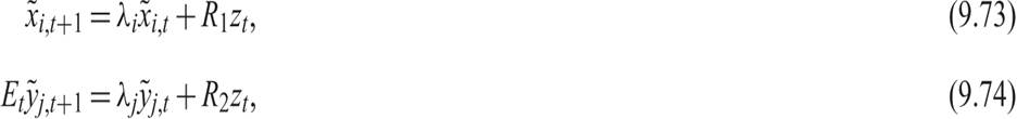
for i = 1, 2, …, n, j = 1, 2, …, m; λ_i is the eigenvalue corresponding to the predetermined variable i; and λ_j is the eigenvalue corresponding to the non-predetermined variable j. The equations (9.73) are solved backward, and the equations (9.74) are solved forward.

9.5.2 Other Solution Methods

The Klein [2000] and Sims [2002] solution methods are variations of the Blanchard and Kahn [1980] solution method. In the Klein [2000] solution method, z_t is assumed to be a zero-mean vector autoregression. The solution method uses a Schur decomposition of the matrices A₁ and A₂, in (9.69) but is otherwise similar to Blanchard and Kahn [1980].

In the Sims [2002] solution method, the rational expectations variables are replaced by their observed values minus their innovation error. No distinction is then required between predetermined and non-predetermined variables. This solution method is based on so-called QZ factorizations of the matrices A₁ and A₂ in (9.54), which, for the Sims solution method, is rewritten as

where e_t+1 = y_t+1 − E_ty_t+1.

Other solution methods rely on a generalization of the method of undetermined coefficients by McCallum [1983], Binder and Pesaran [1995], Uhlig [1999], and Christiano [2002]. Various perturbation methods, also appropriate for nonlinear models, were introduced by Judd [1998], Schmitt-Grohe and Uribe [2004], and others.

9.5.3 A Second-Order Example of the Blanchard-Kahn Method

Let us return now to the share price determination model and see how it can be solved using the Blanchard-Kahn method. The model is the one discussed in section 9.4.3, in which dividends depend on the share price of the previous period. It is described by (9.63) and (9.64). These equations can be rewritten as

alt=eq9-76-77.png>

where (9.64) has been shifted forward one period.

The system of (9.76) and (9.77) can be written in matrix form as

Equation (9.78) has the form of (9.70) of the general Blanchard Kahn model.

which implies that

This is identical to the characteristic polynomial corresponding to the second-order difference equation (9.65). One can show that the characteristic polynomial (9.80) has two roots (say, λ and μ), which lie on either side of unity. The roots satisfy λ + μ = 1 + r, and λμ = δ, where λ is assumed to be the smaller root.

The Jordan decomposition of the coefficient matrix is given by

Thus, the model in (9.78) can be rewritten as

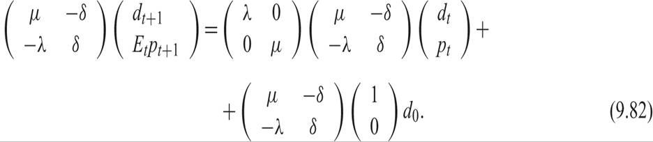
By defining

we can rewrite (9.82) as

Equation (9.83) is a decoupled system of difference equations that can be solved. Once the solutions are obtained, one can use the definitions in (9.83) to solve for p_t and d_t, noting that

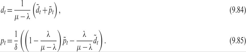
This completes the solution.

9.6