Second-Order Linear Expectational Models
We next turn to the methods of solving a second-order dynamic stochastic linear model under rational expectations. In this model, we assume that an endogenous variable y depends on the rational expectation of its future value yt+1, an exogenous stochastic variable x, and also on its own lagged value yt−1.
This model combines rational expectations about the future value of the variable with the impact of lagged values of the variable. As we shall see in future chapters, the model often arises in macroeconomics. Our model is linear and takes the form
where a, b > 0, and a + b < 1.
This model, which is essentially a second-order difference equation, can be solved using either the factorization method or the method of undetermined coefficients. Of course, both methods result in the same fundamental solution.
9.4.1 The Method of Factorization
Using the future expectations operator F, (9.46) can be written as

where F−1, the inverse of the future expectations operator, is the same as the lag operator.
Moving all terms that contain y to the left-hand side, we get

The left-hand side of (9.48) can be multiplied and divided by − F/a, which results in

This can be rewritten as

Equation (9.49) can be factorized as

where λ and μ are the two roots of the characteristic polynomial of

From (9.50), we know that λ + μ = 1/a, λμ = b/a.
It is simple to show that one root is smaller than unity, and the other is greater than unity. The characteristic polynomial of (9.51) is given by
To show that one root is smaller than unity, calculate the characteristic polynomial for ϕ = 0 and ϕ = 1:

Hence, there is one root (let us assume it is λ) between zero and one, for which Φ(λ) = 0.
The second root μ is determined by

We have μ > 1, if λ < (b/a). This is actually true, because

Therefore, we have that λ < (b/a) < 1, and μ > 1.
The model is saddlepath stable, as it has one predetermined variable, yt−1 and one non-predetermined variable, the rational expectation Et( yt+1). Dividing both sides of (9.50) by F(μ − F), we get

where the last part of (9.53) makes use of the equality aμ = b/λ. This follows from (9.50). From (9.53), it follows that

which is the fundamental solution of (9.46). As in the case of (9.29), (9.54) suggests that the current value of the endogenous variable y depends on the discounted sum of the expected future values of the exogenous variable x, with a discount factor equal to 1/μ < 1. It also depends on its own lagged value, with a coefficient equal to λ < 1.
The factorization method is perhaps a more effective method of solving equations of the form (9.46) than the method of repeated substitutions.
An alternative is the method of undetermined coefficients.9.4.2 The Method of Undetermined Coefficients
To apply the method of undetermined coefficients, as in the case of the first-order model, we assume that the solution of (9.46) takes the form

with undetermined coefficients ϕ, ψ, and ω. From (9.55), the rational expectation of the future y is given by

Substituting (9.56) in (9.46), we get

Comparing coefficients between (9.57) and (9.55), we can solve for the undetermined coefficients:
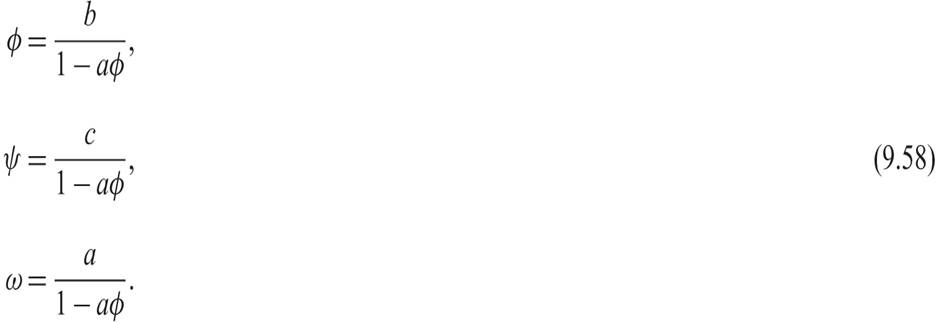
From the first equation in (9.58), ϕ will be the smaller root of the polynomial

This is none other than the characteristic polynomial (9.52), analyzed in the factorization method. There are two roots, λ and μ, where 0 < λ < 1, and μ > 1. The roots satisfy

From (9.58)–(9.60), we get
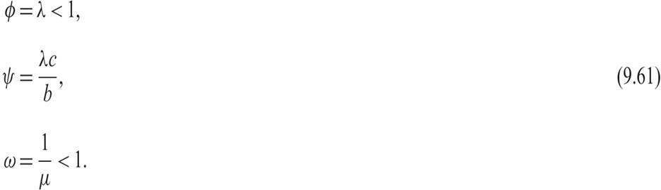
As a result, the fundamental solution is given by

which is the same as (9.54), arrived at through the method of factorization.
9.4.3 An Economic Example of a Second-Order System
As an economic example of a second-order system, we return to the model of the capital market with risk-neutral investors.
Investors choose between a stock and a safe asset with a rate of return r. In equilibrium, arbitrage will ensure that the expected rate of return of the stock will be equal to the rate of return of the safe asset:
where p is the price of the stock, and d is the dividend. The expected rate of return of the stock is equal to the expected capital gain plus the dividend as a proportion of the stock price.
We now assume that the firm has a known dividend policy of the form

where 0 < δ < r. Dividends per share are a constant d0 plus a percentage of the price of the share in the previous period. Presumably this is a policy adopted by the firm and is intended to boost the price of the share.
Substituting (9.64) in (9.63) and solving for the price of the share, we get

Because of the dependence of current dividends on the stock price of the previous period, (9.65) is a second-order equation, like (9.46), with 0 < a = c = 1/(1 + r) < 1, 0 < b = δ/(1 + r) < 1, and a + b < 1. In this case, xt is a constant equal to d0.
Using either the factorization method or the method of undetermined coefficients, the solution of (9.65) gives us the stock price as a function of the past stock price and the constant part of dividends d0:

The two roots λ and μ lie on either side of unity and satisfy λ + μ = 1 + r and λμ = δ. Assume that λ is the smaller root. Note that in the case where δ = 0, we have λ = 0, and μ = 1 + r. With δ = 0, we are back to the first-order case.
One can show from (9.66) and the definitions of the two roots that because d0 is constant, the stock price evolves according to

The stock price converges to a steady state stock price, which is defined by

The steady state stock price is indeed higher than in the case where δ = 0, and the dividend policy of a positive δ does indeed raise the price of the stock.
9.5