Rational Expectations for Linear Autoregressive Processes

We begin with the method for computing the rational expectations solution for the simplest dynamic stochastic model, that of a univariate stochastic process. Exogenous shocks in macroeconomics are often assumed to follow such processes.

Let us assume a variable x, which follows a linear first-order autoregressive stochastic process of the form

where is a constant (the mean of the variable x), and ε is a white noise stochastic process, with zero mean and constant variance.⁵

Define the deviation of x from its mean as

From (9.17) and (9.18) we get that

By repeated substitutions, it is easy to see that

The rational expectation of a first-order linear autoregressive stochastic process depends only on its current value and has a coefficient that depends only on λ.

If the stochastic process (9.17) is stationary (i.e., if., − 1 < λ < 1), then the impact of the current value of the variable on its rational expectation at time t + s is decreasing with s. As s approaches infinity, the limit of the rational expectation is given by

Equations (9.21) and (9.18) imply that

In this sense, the mean of the stationary stochastic process x, which is its long-run equilibrium value, is also the limit to which rational expectations about its future evolution converge over time.

If the process is nonstationary (for example, a random walk for which λ = 1), then (9.20) is transformed to

In this case, the rational expectation for the future value of x is the current value of x, independently of s, as the variable is a random walk and does not converge to a long-run equilibrium.

These methods generalize to higher-order stationary and nonstationary autoregressive moving-average processes.⁶

Exercise 9.1 Compute the rational expectations solution for a second-order, linear, autoregressive process of the form

where a, b > 0, a + b < 1, and ε_t is a white noise process.

How are your conclusions modified if a + b = 1?

9.3 First-Order Linear Expectational Models

We now turn to the rational expectations solution of a linear stochastic model in which a variable y depends on the rational expectation of its future value and on another exogenous stochastic variable x. The model is described by a first-order linear expectational difference equation of the form

The rational expectations hypothesis implies that economic agents know that the variable y is determined by the expectational difference equation (9.24). We also assume that all economic agents have access to the same information set.

Various methods are available for the solution of (9.24). All methods are based on the law of iterated expectations, which requires that the current expectation of the future expectation of a future value of a variable is nothing more than the current expectation of the future value of the variable. That is,

for z, s ≥ 1, and z ≤ s.

9.3.1 The Method of Repeated Substitutions

The simplest method for solving (9.24) is the method of repeated substitutions, a method that we also used to find the rational expectations for the simple first-order autoregressive process in the previous section. From (9.24) and (9.25), we have

Substituting (9.26) in (9.24), we get

Repeatedly substituting the future expectations of y, for T future periods, we get

To have convergence of the last term of (9.27) as T tends to infinity, the absolute value of a must be less than one, and the expected value of x should not increase too quickly. If the expected value of x increases exponentially, its growth rate should not exceed (1/a) − 1. Under these conditions, it follows that

Then a solution of (9.24) can be derived from (9.27):

Note that (9.29) satisfies the condition (9.28) and is thus a solution of (9.24). It suggests that the current value of the endogenous variable y is the discounted sum of the expected future values of the exogenous variable x, with a discount rate equal to a. This solution is usually called the fundamental solution.

However, note that (9.29) is not the only solution of (9.24). The fundamental solution is based only on the minimum number of variables (x in our case), the so-called fundamentals, and satisfies (9.28). If (9.28) is not satisfied, then there exist a host of other, nonfundamental, solutions.

Suppose there is an alternative solution to (9.24) that consists of (9.29) plus an additional variable z.

One can easily demonstrate that if the variable z satisfies

or equivalently,

then (9.30) is also a solution of (9.24).

However, because a < 1, the mathematical expectation of the future z explodes over time. This can be proven by taking the limit of the mathematical expectation as time tends to infinity:

depending on whether z is positive or negative.

Solutions based on nonfundamental variables such as z are called bubbles, as opposed to solutions like (9.29), which are based only on the fundamentals. In the rest of this and in most subsequent chapters, we will focus on the fundamental solutions, ignoring bubbles. We shall return to bubbles in chapter 22.

Besides the method of repeated substitutions, two other methods can be used to solve (9.24): the method of factorization and the method of undetermined coefficients. These methods are simpler to use in more complex dynamic models, for which the method of repeated substitutions soon becomes unwieldy. However, we can also apply them to the simple case of (9.24).

9.3.2 The Method of Factorization

The factorization method requires the use of the future mathematical expectations operator F. We define the future mathematical expectations operator F for a variable x, as

for s = …, − 1, 0, 1, 2, …. Note that this operator is conditional on the information set available in period t, which does not change when the operator is raised to different powers.

It follows that for s = 0, Fx_t = x_t; for s = 1, Fx_t = E_tx_t+1, F²x_t = E_tx_t+2, and so forth.

Using the future mathematical expectations operator and assuming that − 1 < a < 1, (9.24) can be written as

Equation (9.31) is the same as the fundamental solution (9.29) that we found using the method of repeated substitutions. Hence, using the factorization method, one can arrive at the fundamental solution in a few simple steps.

9.3.3 The Method of Undetermined Coefficients

The method of undetermined coefficients consists of using a presumed functional form of a solution with undetermined coefficients, obtaining the mathematical expectation of the presumed solution, replacing this for the expectation in (9.24), and comparing the coefficients of the resulting equation with the undetermined coefficients of the presumed solution. If the form of the presumed solution is correct, this method will suffice to determine the undetermined coefficients.

For example, if our guess is that the solution has the form

where σ and μ are undetermined coefficients, then

Substituting (9.33) in (9.24) and comparing coefficients between the resulting equation and (9.32), we find that σ = b and μ = a. This confirms our presumption of (9.32), and the solution is exactly the same as with the two other methods.

The choice of method to be used to solve models with rational expectations depends on the ease of application.

9.3.4 Two Additional Economic Examples

To see how these methods are applied, we shall use two simple economic models that result in equations of the form (9.24).

Stock Prices in Efficient Capital Markets In our first model, we assume a capital market in which investors are risk neutral. They choose between a common stock with an uncertain return and a safe asset with a certain rate of return r. In equilibrium, arbitrage will ensure that the expected rate of return of the stock will be equal to the rate of return of the safe asset:

where p is the price of the stock in the capital market, and d is the dividend. The expected rate of return of the stock is equal to the expected capital gain plus the dividend as a proportion of the stock price. In equilibrium in an efficient capital market, this cannot differ from the rate of return of the safe asset r. Equation (9.34) can be rearranged as

which has the form of (9.24), with 0 < a = b = 1/(1 + r) < 1.

The solution of (9.35) gives us the stock price as a function of expected future dividends:

Thus, the stock price is the present value of the current and expected future dividends, discounted by the rate of return of the safe asset.

The Cagan Model of Money Demand In our second model, we assume that consumers and firms decide between holding money and goods in the face of inflation. Money is a nominal asset whose real value is affected negatively by inflation. In this case, the demand for money is a negative function of expected inflation, and money market equilibrium requires that

where M is the nominal money supply, P is the price level, and α > 0 is the semi-elasticity of money demand with respect to expected inflation. This model was first used by Cagan [1956] to explain hyperinflation.⁷

Taking logarithms on both sides and denoting the logarithm of the nominal money supply by m and the logarithm of the price level by p, the model can be written in log-linear form as⁸

Solving for p_t results in

Equation (9.39) has the form of (9.24), with

The fundamental solution takes the form

The current price level depends on the discounted expectations about the evolution of the money supply in the future, with a discount factor equal to 0 < α/(1 + α) < 1. Thus, it is the full expected future path of the money supply, and not just the current money supply, that determines the price level in this model.

9.3.5 Alternative Assumptions about the Evolution of Exogenous Variables

The solution of equation (9.24) (for example, (9.29)) is based on the discounted rational expectations about the future path of the exogenous variable x. To have a closed-form solution for the variable y, we must make additional assumptions about the evolution of the exogenous variable x. The final closed-form solution depends on such assumptions.

We shall examine two alternative examples to demonstrate this point.

Our first assumption is that the exogenous variable x is expected to remain constant at the level x₀. From (9.29), the endogenous variable y is determined by

This is the assumption usually made in deterministic models with perfect foresight, such as the growth models of chapters 3–8. If x changes permanently and unexpectedly from x₀ to x₁, then y jumps immediately from the initial equilibrium value, y₀ = (b/(1 − a))x₀, to the new equilibrium value, y₁ = (b/(1 − a))x₁. Equation (9.41) can also be used to analyze the impact of an anticipated future change in the constant level of the exogenous variable.

Let us assume that at time t₀, it is announced that from a future period t₁ onward, the variable x will rise from x₀ to a new constant level x₁. In this case, the path of the endogenous variable y will be as follows:

At the time of the announcement t₀, variable y jumps up, as the expectations about the future path of x change. Until the change is implemented at time t₁, y continues rising gradually, as the impact of the higher x₁ after period t₀ rises, compared to the impact of the lower x₀ in the interval t₁ − t. After period t₁, the endogenous variable y is stabilized at the higher level corresponding to the higher x₁.

If x is the dividend, as in our first example, then the share price will rise immediately after the announcement of a future dividend increase and will continue rising as the expected dividend increase approaches. When the increase in the dividend materializes, the stock price stops growing and is stabilized at the new higher level, corresponding to the higher dividend.

If x is the money supply, as in our second example, the price level will rise immediately after the announcement of a future increase in the money supply, and it will continue rising until the rise in the money supply materializes. The price level will then be stabilized at its new higher level.

The second case that we analyze is based on the assumption that the exogenous variable x follows a first-order linear autoregressive stochastic process, as in (9.17). In this case, we have

which converges to

Thus, (9.42) can be written as

where is the steady state value of y.

This case is relevant for stochastic models, such as the models examined in this and subsequent chapters, and especially the models of aggregate fluctuations in chapters 13–22.

In the stock price model, (9.43) tells us that the price of the stock will be a function only of the current dividend. This is because if dividends follow a first-order autoregressive stochastic process (as we have assumed), the current dividend is the only element required to predict future dividends. Because dividends follow an AR(1) process, the price of the stock will also follow an AR(1) process.

Similarly, in the money demand model, (9.43) tells us that the price level will be determined only by the current money supply. This is because if the money supply follows a first-order autoregressive stochastic process (as assumed), the current money supply is the only element required to predict the future course of the money supply.

Exercise 9.2 Derive and discuss the rational expectations solution of the stock market model and the money demand model, assuming that the dividend and the money supply process follow a second-order autoregressive process of the form

where denotes either the deviation of the dividend (in the stock market model) or the money supply (in the money demand model) from its long-run equilibrium level. Assume that a, b > 0, a+b < 1, and ε_t is a white noise process. How is your solution modified if a + b = 1?

9.3.6 The Expectational Competitive Market Model Revisited

Returning to the expectational competitive market model of section 9.1, let us assume that the supply shock v_t follows a first-order autoregressive process of the form

where 0 < λ < 1, and ε_t is a white noise process. Then, from (9.16) and (9.44), the closed-form rational expectations solution for the equilibrium price is given by

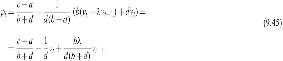
The current supply shock depresses the equilibrium price, as it increases current supply. But the past supply shock boosts the price, because by positively affecting prior expectations about the current supply shock, it induces firms to reduce supply, as it reduces their expectation about the current price. Note that the dynamics of the market price differ from the case of adaptive expectations in equation (9.11), and there is no cobweb pattern in this case either.

9.4