A Stochastic Expectational Model of a Competitive Market
In this section, we consider a simple expectational model of a competitive market to illustrate the differences between deterministic and stochastic models and to highlight the importance of the treatment of expectations.
This is a log-linear model, in which demand is a function of the current price, but supply decisions are made one period in advance, based on the prior expectations of firms for the current price. Hence, the expectations about the current price, based on information available one period in advance, partly determine the supply of the commodity in question. In addition, there is a stochastic supply shock, which cannot be known in advance. Ex post, the market clears at a price that equates this partly predetermined supply with current market demand.
This simple expectational model, known as the cobweb model because of its dynamic properties under adaptive expectations, has played a very important role in the study of market cycles and expectations in economics.3
The model consists of log-linear demand and supply functions, and an equilibrium condition requiring that the current price adjusts to equate demand and supply.
The supply of the commodity is question is determined by

where  denotes the logarithm of the supply of commodity Q in period t, and
  is the expectation of suppliers about the logarithm of the market price at t, based on information they possess in the previous period t − 1. In addition, a and b are constant positive parameters, and vt is a stochastic supply shock.
The demand for the commodity is determined by

where  denotes the logarithm of the demand for commodity Q in period t, pt is the logarithm of the market price at t, and c and d are constant positive parameters. It is assumed that demand is a negative function of the current price; d is the elasticity of demand with respect to the current price.
The market being competitive, equilibrium is determined by the equality of demand and supply. Thus, the equilibrium condition is that

where qt is the equilibrium quantity.
From (9.1)–(9.3), the equilibrium price is determined by

From (9.4), the equilibrium price depends negatively on the prior expectation of the equilibrium price by suppliers. The higher the expected price is the higher the supply will be, and therefore the lower the resulting equilibrium price will be. To solve for the market equilibrium in terms of the market fundamentals (like the parameters a, b, c, d, and the supply shock vt), we must make an assumption about the formation of expectations.
9.1.1 Absence of Uncertainty and Perfect Foresight
If there is no uncertainty, and suppliers know the supply shock with certainty, a natural assumption about the formation of expectations in this case is the assumption of perfect foresight. In fact, this is the assumption we have been utilizing in the optimizing deterministic models of chapters 2–8.
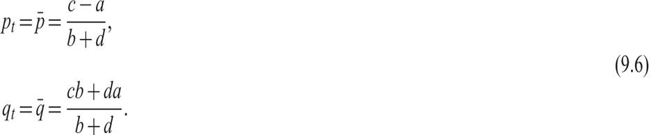
Because everybody knows everything with certainty, suppliers can form a perfect prediction of the equilibrium price, and in this case, . Hence, equilibrium prices and quantities under perfect foresight are given by
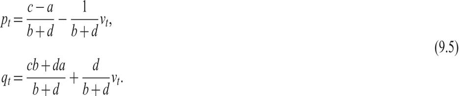
Because there is no uncertainty about either the parameters a, b, c, d or the supply shock vt, suppliers can forecast the equilibrium price perfectly, and the model becomes equivalent to a simple demand and supply competitive model, in which the price moves immediately to clear the market.
If vt is a random variable or a stochastic process, the model is stochastic, and prices and quantities fluctuate randomly, as they are driven by the stochastic process followed by the exogenous supply shock vt. Otherwise, the model is deterministic. For example, in the case of a deterministic model where the supply shock is constant and equal to zero, equilibrium prices and quantities are also constant:
9.1.2 Uncertainty and Adaptive Expectations
What if there is uncertainty about the evolution of the supply shock vt? Then suppliers, not knowing the market price, which will depend on the unknown supply shock, will have to form expectations about the price in advance.
The key hypothesis traditionally made about the formation of expectations under uncertainty is the hypothesis of adaptive expectations.
The adaptive expectations hypothesis is an empirically motivated short-cut to the formation of expectations, postulating that agents adapt their expectations gradually to correct for past expectational errors. It was the key expectational hypothesis for many decades before the appearance of the rational expectations hypothesis.
In the context of our simple competitive model, the adaptive expectations hypothesis postulates that supplier’s expectations about the market price evolve according to

Equation (9.7) implies that if the equilibrium price in the previous period was higher than the previously expected equilibrium price, the expected equilibrium price for next period will be revised upward. In the equation, 0 ≤ λ ≤ 1 measures the degree of inertia in the revision of expectations. If λ = 1, there is full inertia, and expectations are never revised. This is the case of static expectations, implying that  for all t. If λ = 0, there is no inertia, and expectations are fully revised and are therefore equal to the previous price. In the context of our model, this case of fully adaptive expectations implies that

Substituting the fully adaptive expectations hypothesis (9.8) for the expected price in the expectational equilibrium price equation (9.4), we get that the equilibrium price is determined by

This is a stochastic first-order difference equation that determines the equilibrium price as a negative function of the previous equilibrium price. In the absence of shocks, the equilibrium price will display oscillations. High prices today cause an increase in supply and low prices tomorrow, and vice versa. It was this type of behavior of prices (and quantities) that led Kaldor [1934] to name this model the cobweb model, as the diagrammatic representation of this type of price and quantity adjustment looks like a cobweb.
This cobwed is depicted in figure 9.1.
The pair of equilibrium price and quantity, if the expectations of suppliers are correct, is determined at point E and is given by (pE, qE). If, however, the initial price in period 0 is equal to p0, above the equilibrium price, supply in period 1 will be equal to q1, above the equilibrium quantity. For this higher quantity to be sold, the price in period 1 must fall to p1, which is below the equilibrium price. At the low p1, the quantity supplied in period 2 will fall below the equilibrium quantity, at q2, prompting the price to rise above the equilibrium price in period 2. The process will continue, and in the example shown in figure 9.1, prices and quantities will eventually converge, in a cobweb fashion, to the equilibrium pair (pE, qE).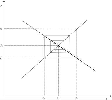
Figure 9.1 The cobweb model under adaptive expectations.
In the absence of supply shocks, the oscillations will lead to convergence to an equilibrium price only if the root of the difference equation (9.9) is less than unity in absolute terms:

This condition requires that the elasticity of supply with respect to the expected price b is lower (in absolute terms) than the elasticity of demand with respect to the current price d. If the elasticities are equal, there will be nonconvergent oscillations; if the supply elasticity exceeds the demand elasticity, the oscillations will diverge, and the model will be unstable.4
In general, in the presence of supply shocks, and if (9.10) is satisfied, the solution of the difference equation (9.9) takes the form

Equilibrium prices (and quantities) are a geometrically distributed lag of current and past supply shocks, with alternating signs.
If the supply shocks are stochastic, equilibrium prices and quantities will be stochastic as well. It is important to note that current prices and quantities are backward looking, because of the assumption of adaptive expectations, which make future expectations a function of past prices.9.1.3 The Rational Expectations Hypothesis
The rational expectations hypothesis was introduced by Muth [1961], who illustrated its significance using a version of the particular expectational market model introduced in section 9.12.
Muth [1961, p. 316] argued that
expectations, since they are informed predictions of future events, are essentially the same as the predictions of the relevant economic theory. …we call such expectations “rational.” …The hypothesis can be rephrased a little more precisely as follows: that expectations of firms (or, more generally, the subjective probability distribution of outcomes) tend to be distributed, for the same information set, about the prediction of the theory (or the “objective” probability distributions of outcomes).
Rational expectations are thus defined as the mathematical expectations for the future evolution of a stochastic variable, based on the model determining this variable and a given information set.
Thus defined, the rational expectation of a variable x in period t + 1, based on available information in period t, is the mathematical expectation of the variable at t + 1, conditional on the information set available at t:

where

Here It is the set of available information, which consists of current and past values of the variable x itself, as well as the current and past values of a set of variables z, which affect and thus can help predict the future values of x. Note that this definition of the information set does not involve loss of memory, as whatever is known in period t is also known in period t + 1 and all future periods.
More generally, we define the rational expectation of a variable x at t + s, based on available information at t, as

In what follows, let us simplify the notation by using Etxt+s in place of E(xt+s|It).
Note that to define rational expectations for a variable more precisely, it is not enough to specify the information set. One also needs to specify the model determining how this variable evolves over time.
Imposing the rational expectations hypothesis on our competitive market model implies that the formation of expectations about prices will take account of the price determination process itself. Hence, expectations will be formed taking into account the price determination equation (9.4).
Applying the rational expectations hypothesis to (9.4), by taking the rational expectation of the market price conditional on information available up to period t − 1, implies that

Hence, the rational expectation of the equilibrium price is equal to the equilibrium price in the absence of supply shocks, adjusted for the rational expectation of the impact of the supply shock, based on information available in period t − 1.
Substituting for this rational expectation in the expectational price equation (9.4), we have that the equilibrium price is given by

Supply shocks depress the equilibrium price, because they increase supply relative to demand. However, to the extent that the shocks are unexpected, they have an additional depressing effect, because suppliers have overestimated the equilibrium price and hence have increased supply by more than they would have done otherwise.
In the case where supply shocks are fully expected, there are no unanticipated shocks, and we are back to the perfect foresight case described by (9.5). In the case where supply shocks are fully unexpected, the rational expectations solution takes the form

The unexpected supply shock reduces the equilibrium price, but there is no cobweb pattern.
The rational expectations solution in general differs from the solution under adaptive expectations, as it does not depend on the whole history of past supply shocks but only on whatever information is required at t − 1 to form a rational expectation of the supply shock in period t. In addition, there is no cobweb under rational expectations, as expectations about current prices do not depend only on past prices, as postulated by the adaptive expectations hypothesis. However, to fully solve the model under rational expectations, we need to assume a model for the evolution of the exogenous supply shock vt. This model will be the one used to calculate the rational expectation of prices on the basis of past information.
We have already solved the model for perfectly anticipated and perfectly unanticipated supply shocks. In the case of partly anticipated supply shocks, one has to make specific assumptions about the stochastic process determining the evolution of such shocks. Let us postpone this discussion until we examine how rational expectations of a stochastic process are computed. We thus turn to the discussion of solution methods for more general stochastic models of exogenous shocks and more general dynamic stochastic models under rational expectations.
9.2