Optimal Investment under Uncertainty
We now turn to the case of investment under uncertainty. As in the case of consumption, uncertainty introduces additional problems. Just as under certainty, we shall assume that the firm chooses its investment path to maximize its value to its owners.
The value is equal to the present value of the profits that the firm generates.11.2.1 The Value of a Firm under Uncertainty
Under certainty, the problem of maximizing the present value of the profits of the firm is easily defined. But under uncertainty, the question that arises is: What is the discount rate at which firms should discount future profits?
Let us assume that 𝒱t is the value of the firm in period t, and 𝒫t is its per period revenue, net of investment expenditures. Then the rate of return 1 + πt from holding the firm for one period is given by

For a household that invests in the firm under uncertainty, the rate of return from holding the firm 1 + πt, and hence Vt and Πt, must satisfy

Equation (11.15) is similar to the first-order condition (10.12) for investing in a risky asset in the problem analyzed in chapter 10. The returns generated by the firm in each state of nature are weighted by the marginal utility of consumption in that state. The discount factor that must be applied must take into account the correlation of the firm’s profits with the marginal utility of consumption at each state.
Solving the first-order condition (11.15) recursively forward and assuming away bubbles, we get the fundamental solution for the value of the firm 𝒱t:

This equation shows that the value of the firm is equal to the present discounted value of expected future profits.
The discount rate for each period and for each state of nature is the marginal rate of substitution between consumption at time t and consumption at that period and that state of nature. The implication is that the higher the correlation between a firm’s profits and consumption is, the higher will be the discount factor applied and the lower the value of the firm.In practice, it is often assumed that firms maximize the present discounted value of profits by using a deterministic discount rate. For firms opting to do this, (11.16) becomes

where rt+z is a deterministic interest rate in period t + z. Although widely used, a specification such as (11.17) is generally inappropriate, because it suggests that at each date, the same discount factor is used to evaluate returns in different states of nature.
An equation such as (11.17) can be justified only under very specific assumptions. One assumption that can be used to justify it is the assumption of risk neutrality on the part of consumers. If consumers are risk neutral, so their utility is linear in consumption and their marginal utility of consumption is constant, then the discount rate is not only deterministic but also constant, and it equals the pure rate of time preference ρ. Thus, in the case of risk neutrality, (11.17) simplifies further to

Another set of assumptions that can be used to justify a deterministic discount rate is to assume that investment decisions do not affect the relative distribution of returns across states of nature but only the scale of the firm. In this case, the firm can use a constant discount rate, equal to the risk free rate, plus a risk premium that reflects the specific risk associated with the firm’s activities.
Both sets of assumptions are unlikely to hold in general, but they are often used as convenient approximations.
However, they are good approximations only when considerations of risk aversion are not central to the problem analyzed.11.2.2 The Lucas-Prescott Model of Investment under Uncertainty
We next turn to an examination of the investment decisions of a competitive firm under uncertainty, assuming that the objective of the firm is to maximize value as defined in (11.18), with a deterministic discount rate. The model we analyze is a linear quadratic variant of the class of models introduced by Lucas and Prescott [1971]. It is similar in many respects to the q model analyzed in section 11.1.
Assume a competitive firm i that takes market prices as given. Its profit in period t is defined by

where p is the competitive relative price of its output Y; I is gross investment; and ψ is a constant positive parameter measuring the strength of investment adjustment costs, which are quadratic in gross investment. The relative price of investment goods is normalized to unity.
Output is produced using capital, through a linear production function of the form

where A is total factor productivity, assumed to be constant and the same for all firms.
The relation between gross investment and the evolution of the capital stock is determined by

where δ is the constant depreciation rate, and i is uniformly distributed in the interval [0, 1]. Thus, industry output is given by

Because all firms face the same technology and the same market prices, the output of all firms will be the same. Thus, from now on, we treat Y as the output of the representative firm.
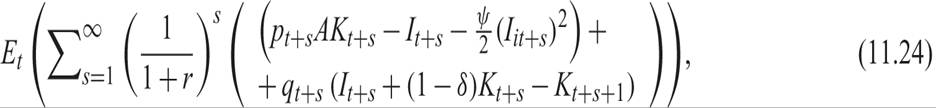
The same goes for all other variables, such as investment and the capital stock.Under the assumptions we have made, the representative firm maximizes its expected present value

subject to the sequence of accumulation equations (11.21). The stochastic processes driving the market price and productivity are taken as given.
The Lagrange function of this problem is defined by
where qt+s is the sequence of Lagrange multipliers of the capital accumulation constraints.
From the first-order conditions for a maximum, we get the two familiar first-order conditions:
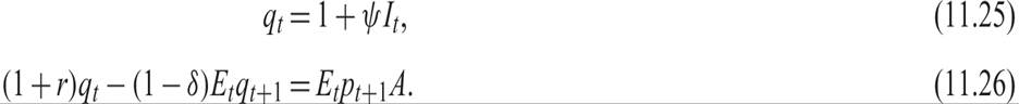
Equations (11.25) and (11.26) have interpretations similar to the that of the corresponding conditions (11.7) and (11.8) in the deterministic case analyzed in section 11.1. Equation (11.25) requires that at the optimum, the firm equates the shadow value of an addition to its capital stock q to the marginal cost of investment. The latter consists of the price of purchasing capital goods (assumed to be equal to one) plus the adjustment cost of investment.
Equation (11.26) requires that the user cost of capital, as measured by the term on the left-hand side, is equal to the expected future value of the marginal product of capital, as measured by the term on the right-hand side. Solving (11.26) forward for q, we get

So q turns out to be the discounted value of all expected future values of the marginal product of capital. It depends positively on the expected future evolution of the relative price for the product of the firm and the marginal productivity of capital A.
It also depends negatively on the discount rate r and the depreciation rate δ.To determine investment, we can solve (11.25) for investment:

From (11.28), investment depends positively on the difference of q from unity, which is the purchase price of investment goods. Substituting (11.27) in (11.28), investment of the representative firm will be determined by

Investment thus depends positively on the discounted value of all expected future changes in the value of the marginal product of capital; it depends negatively on the real interest rate, the depreciation rate, and the adjustment cost parameter ψ.
From (11.29), the capital stock of the representative firm evolves according to

To say more about the determination of investment and the capital stock, one must make specific assumptions about the stochastic process driving the market price of output.
Although for each competitive firm, the price of output is taken as given, for the industry, the market price will be determined endogenously from the equation of total demand for its product and industry supply. Industry supply will depend on investment and the evolution of the capital stock. This is something that Lucas and Prescott [1971] took explicitly into account, solving for the equilibrium price endogenously as a function of the capital stock, and characterizing the evolution of the capital stock and the equilibrium price in a rational expectations equilibrium.
11.2.3 Rational Expectations Equilibrium and Aggregate Investment in the Lucas-Prescott Model
Assume that industry demand is linear in the price and is given by

where D > 0, b > 0 are constant parameters; D measures the size of the market; b the price responsiveness of demand; and v is a stochastic disturbance to industry demand.
From (11.31), and after substituting for output from the production function, the competitive (relative) price is determined as

We can use (11.32) to substitute for the expected equilibrium price in the capital accumulation equation (11.30) and solve for the evolution of the capital stock as a function of only exogenous shocks.
Note that using the forward shift operator, Fpt = Et(pt+1), (11.30) can be written as

The above can be rewritten as

Multiplying both sides of (11.33) by (1 + r) − (1 − δ)F and collecting the terms containing K on the left-hand side, after using (11.32) to substitute out for pt, we get
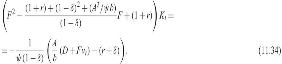
The characteristic polynomial of the quadratic equation involving F on the left-hand side has two roots that lie on either side of unity. We can thus rewrite (11.34) as

where λ < 1 is the smaller root, and μ > 1 the larger root. It follows from (11.34) that λ = (1 + r)/μ, as the roots satisfy

From (11.35), the capital stock follows:
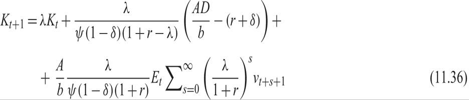
Equation (11.36) shows that the evolution of the industry capital stock in rational expectations equilibrium depends on current expectations about the whole future path of disturbances to industry demand and on parameters such as the discount rate r, the productivity of capital A, the adjustment cost parameter ψ, the depreciation rate δ, the size of the market D, and the price responsiveness of industry demand b. The root λ depends only on the discount rate and technological parameters.
To get a closed-form solution, we must make assumptions about the exogenous stochastic process driving industry demand. Assume that v follows a stationary AR(1) process of the form

where 0 < θ < 1, and εt is a white noise process.
Under this assumption, (11.36) implies that


Investment and the evolution of the capital stock depend only on the current shock to aggregate demand, because the current shock is a sufficient statistic for all future shocks to industry demand.
Thus, the structure of the full Lucas-Prescott model is as follows. The representative firm chooses investment—and implicitly, the capital stock and output—to maximize the present value of its profits, taking as given the market price of its output, the exogenous relative price of capital goods, and exogenous productivity A. To compute the full equilibrium, once investment and output of the representative firm are determined, industry output is replaced in the industry demand function to solve for the equilibrium price in terms of the exogenous stochastic process driving industry demand. The full rational expectations equilibrium is thus described by a pair of interrelated capital accumulation and price equations, which are consistent with continuous market clearing in a competitive industry.
This model can be ammended in various directions. First, one could introduce additional shocks, such as shocks to total factor productivity. Second, one could introduce labor in the production function and study interactions between investment and labor demand. Third, one could introduce business taxes. Fourth, one could introduce externalities from capital accumulation. Finally, one could assume imperfect rather than perfect competition.4
11.3