Optimal Investment with Convex Adjustment Costs

Let us consider a competitive firm producing a good Y. The production function of the firm is given by

where A is total factor productivity, and K is the capital stock.

To change its capital stock, the firm must undertake gross investment I. The change in its capital stock is thus determined by

where δ is a constant depreciation rate.

Assume that the instantaneous cost of gross investment for the firm is equal to

where ψ is a convex function, for which it holds that ψ(0) = 0, ψ′ > 0, and ψ′′≥ 0. The convex function ψ measures the installation (adjustment) cost of gross investment. It is assumed that the higher the size of gross investment is, the higher the marginal installation cost will be. The total cost of gross investment is thus equal to the cost of buying the relevant capital goods plus the installation (adjustment) cost.

Figure 11.1 depicts the adjustment (installation) cost as a function of the size of gross investment of the firm. The installation cost rises as the absolute volume of gross investment rises. If the second derivative is positive, the installation cost rises at an increasing rate. The adjustment cost function is assumed symmetric. Thus, what applies to positive investment also applies to negative investment. The instantaneous profits of the firm are thus equal to

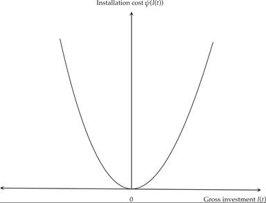
Figure 11.1 Adjustment cost of investment.

11.1.1 The Choice of Optimal Investment

Assume that at time 0, the firm chooses an investment path that maximizes the present value of current and future profits. Assuming an infinite time horizon, the present value of the profits of the firm is equal to

where r is the real interest rate, assumed exogenous and constant. The present value (11.5) is maximized under the constraint of the production function (11.1) and the investment function (11.2), which links gross investment to the accumulation of capital.

The current-value Hamilton function of this problem is defined by

where q(t) is the multiplier of the capital accumulation constraint (11.2) and represents the shadow value of an additional unit of capital at instant t.

From the first-order conditions for a maximum, it follows that

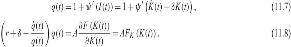
The interpretation of this form of the first-order conditions is straightforward. Condition (11.7) determines the optimal shadow value of an additional unit of capital q as equal to the marginal cost of investment. This is equal to the purchase price of capital goods (assumed equal to unity) plus the marginal installation (adjustment) cost ψ′(I(t)).

Condition (11.8) requires that at the optimum, the firm will invest until the user cost of capital (on the left-hand side) is equal to the marginal product of capital (on the right-hand side). The user cost of capital is the real interest rate, plus the depreciation rate, minus the expected appreciation rate of the capital stock, all multiplied by the shadow value of capital q(t).

11.1.2 The Case of Zero Adjustment Costs

In the case of zero adjustment costs, the marginal adjustment cost of the capital stock ψ′ is equal to zero.

These are the usual first-order conditions that we have utilized so far. The variables q and K jump immediately to their equilibrium values. The shadow value of capital is continuously equal to unity (i.e., the purchase price of capital goods and the capital stock adjust immediately to the level where the marginal product of capital is equal to the real interest rate plus the depreciation rate, r + δ). There is no investment flow, as the capital stock adjusts immediately. Without adjustment costs, this model does not determine gross investment but only the equilibrium capital stock.

11.1.3 The Investment Function with Convex Adjustment Costs

Let us now return to the general case, where there is a strictly convex adjustment cost function for the capital stock. From (11.7), it follows that investment is a positive function of q − 1. Solving (11.7) for I, we get

Gross investment depends only on the difference of the shadow price of installed capital q from unity, as assumed by Tobin. This dependence is positive, because the marginal cost of investment is positive. For this reason, the theory that depends on rising adjustment costs of investment is referred to as the q theory of investment.

11.1.4 The Determinants of q

We have already defined q as the shadow price of an additional unit of installed capital. We next turn to the determinants of q. From the first-order condition (11.7), q is equal to the marginal cost of investment. We have already used this condition to derive the investment function (11.9).

To analyze the determinants of q, we must look into the second first-order condition (11.8). This can be rewritten as

Equation (11.10) is a first-order linear differential equation with variable coefficients.

From (11.11), it follows that q is the present value of all future marginal products of capital. As a result, q depends negatively on the real interest rate and the depreciation rate, as well as on factors that reduce the marginal product of capital (such as the capital stock). In contrast, q depends positively on factors that increase the marginal product of capital (such as total factor productivity).

In equilibrium, q is determined so that both first-order conditions are satisfied. Thus, in equilibrium, the marginal cost of investment is equal to the expected present value of future marginal products of capital. This condition determines optimal investment.

11.1.5 Dynamic Adjustment of q and the Capital Stock K

The determination of the shadow price of an additional unit of capital q, and the stock of capital K, can be inferred from the differential equations (11.7) and (11.8). Because both of these differential equations are nonlinear, their solution can be described by a phase diagram, as in figure 11.2.

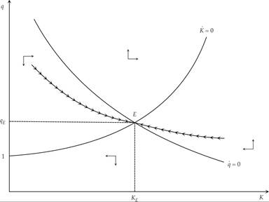
Figure 11.2 Determination of q and the capital stock K.

For a constant capital stock, (11.7) implies that

The higher the stock of capital is, the higher will be the shadow value q implied by (11.12), as depreciation investment will be higher. Equation (11.12) is depicted as the curve with a positive slope in figure 11.2 and can be interpreted as the constant capital stock condition. When q is higher than the level implied by (11.12), the capital stock increases, as gross investment is higher than depreciation investment. The opposite happens when q is lower than the level implied by (11.12): Then the capital stock decreases.

For a constant q, (11.8) implies that

so, the higher the stock of capital is, the lower the shadow value of capital q will be, as the marginal product of capital is a negative function of the stock of capital. Equation (11.13), which is the curve with a negative slope in figure 11.2, can be seen as the constant gross investment condition. When K (the stock of capital) is higher than the level implied by (11.13), then the marginal product of capital is lower than what would be required by (11.13), and q increases, so that the user cost of capital is also lower. Thus, investment is low but increasing over time. The opposite happens when the capital stock is lower than the level implied by (11.13).

The steady state is determined at the intersection of the two curves (11.12) and (11.13). This steady state equilibrium is a saddle point, because q is a non-predetermined variable and K is a predetermined variable. The adjustment path is unique and is depicted in figure 11.2.

Figure 11.3 shows the effects of a permanent increase in the real interest rate. This leads to increase in the user cost of capital and a downward shift of the constant investment condition. Because the capital stock is predetermined in the short run, the change leads to an immediate reduction of q and investment, and a gradual reduction of the stock of capital. As the capital stock decreases, the marginal product of capital gradually increases, which causes a gradual increase in both q and investment. At the new steady state E′, both the stock of capital and q are at a lower level than at the initial steady state E.

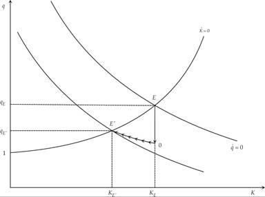
Figure 11.3 Dynamic effects of a permanent rise in the real interest rate.

Figure 11.4 shows the effects of a permanent increase in total factor productivity A, which leads to an increase in the marginal product of capital and a shift upward of the constant investment condition.

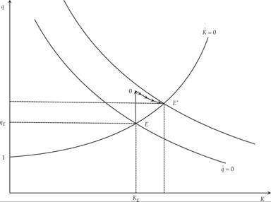
Figure 11.4 Dynamic effects of a permanent rise in total factor productivity.

The dynamics depicted in figures 11.2–11.4 describe the basic neoclassical model of investment with convex adjustment costs. This model can be generalized so that the adjustment cost function depends not only on gross investment but also on the stock of capital. It can also be generalized to simultaneously analyze investment and labor demand. Finally, it can also be generalized to allow for product market imperfections, as well as to the case of uncertainty.

11.2