Overlapping Generations in Continuous Time

9.8.1. Demographics, Technology and Preferences. We now turn to a continuous time version of the perpetual youth model. Suppose that each individual faces a Poisson death rate of ν ∈ (0, ∞).

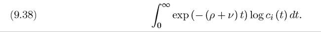
Demographics in this economy are similar to those in the discrete time perpetual youth model of the previous section. In particular, expected further life of an individual is inde­pendent of when he was born, and is equal to

This is both the life expectancy at birth and the expected further life of an individual who has survived up to a certain point. Next, let population at time t be L (t). Then the Poisson death rate implies that a total flow of νL (t) individuals will die at time t. Once again we assume that there is arrival of new households at the exponential rate n > v,so that aggregate population dynamics are given by

again with initial condition L (0) = 1. It can also be computed that at time t the mass of individuals of cohort born at time τ < t is given by

In this equation and throughout the section, we assume that at t = 0, the economy starts with a population of L (0) = 1 who are all newborn at that point. Equation (9.40) is derived in Exercise 9.23.

As in the previous section, it is sufficient to specify the consumption behavior and the budget constraints for each cohort.

time t is

where again z (a (t | τ) | t, τ) is the transfer payment or annuity payment at time t to an individual born at time τ holding assets a (t | τ). We follow Yaari and Blanchard and again assume complete annuity markets, with free entry. Now the instantaneous profits of a life insurance company providing such annuities at time t for an individual born at time τ with since the individual will die and leave his assets to the life insurance company at the flow rate ν. Zero profits now implies that

Substituting this into the flow budget constraint above, we obtain the more useful expression

Let us assume that the production side is given by the per capita aggregate production function f (k) satisfying Assumptions 1 and 2, where k is the aggregate capital-labor ratio. Capital is assumed to depreciate at the rate δ. Factor prices are given by the usual expressions and as usual r (t) = R (t) — δ. The law of motion of capital-labor ratio is given by

where c (t) is average consumption per capita, given by

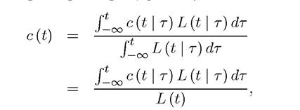
where recall that L (t | τ) is the size of the cohort born at τ at time t.

9.8.2. Equilibrium.

Definition 9.4. A competitive equilibrium consists of paths of capital stock, wage rates

according to (9.43).

Let us start with consumer optimization.

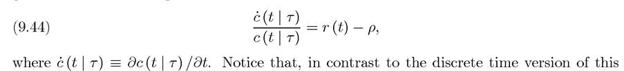
equation, (9.37), the probability (flow rate) of death, ν, does not feature here, since it exactly cancels out (the rate of return on assets is r (t) + ν and the effective discount factor is ρ + ν, so that their difference is equal to r (t) — ρ).

The transversality condition for an individual of cohort τ can be written as

where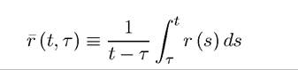

is the average interest rate between dates τ and t as in equation (8.17) in Chapter 8, and the transversality condition here is the analog of equation (8.18) there. The transversality condition, (9.45), requires the net present discounted value of the assets in the very far future of an individual born at the time τ discounted back to this time to be equal to 0.

Combining (9.44) together with (9.41) and (9.45) gives the following consumption “func­tion” for an individual of cohort τ (see Exercise 9.24):

This linear form of the consumption function is a particularly attractive feature of logarithmic preferences and is the reason why we specified logarithmic preferences in this model in the first place. The term in square brackets is the asset and human wealth of the individual, with the second term defined as

This term clearly represents the net present discounted value of future wage earnings of an individual discounted to time t. It is independent of τ, since the future expected earnings of all individuals are the same irrespective of when they are born.

Equation (9.46) implies that each individual consumes a fraction of this wealth equal to

as

where a (t) is average assets per capita. Since the only productive assets in this economy is

The law of motion of assets per capita can be written as

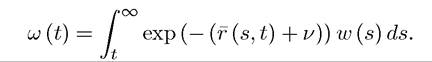
This equation is intuitive. Aggregate wealth (a (t) L (t)) increases because of the returns to capital at the rate r (t) and also because of the wage income, w (t) L (t). Out of this, total consumption of c (t) L (t) needs to be subtracted. Finally, since L (t) grows at the rate n — ν, this reduces the rate of growth of assets per capita. Human wealth per capita, on the other hand, satisfies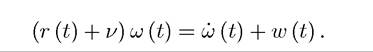

The intuition for this equation comes from the Hamilton-Jacobi-Bellman equations discussed in Chapter 7. We can think of ω (t) as the value of an asset with a claim to the future earnings of a typical individual. The required rate of return on this is r (t) + ν, which takes into account that the individual will lose his future earnings stream at the rate ν when he dies. The return on this asset is equal to its capital gains, ω (t), and dividends, w (t). Now substituting for a (t) and ω (t) from these two equations into (9.48), we obtain:

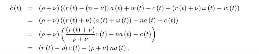
where the third line uses (9.47).

(9.49)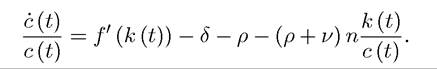

This is similar to the standard Euler equation (under logarithmic preferences), except for the last term. This last term reflects the fact that consumption growth per capita is slowed down by the arrival of new individuals at each instance, who have less wealth than the average individual. Their lower wealth implies lower consumption and reduces average consumption growth in the economy. This intuitively explains why the last term depends on n (the rate of arrival of new individuals) and on k/c (the size of average asset holdings relative to consumption).

The equilibrium path of the economy is completely characterized by the two differen­tial equations, (9.43) and (9.49)—together with an initial condition for k (0) > 0 and the 371

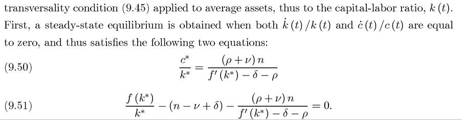
The second equation pins down a unique positive level of steady-state capital-labor ratio, k*, ratio (since both f (k) /k and f⁰ (k) are decreasing). Given k* the first equation pins down a unique level of average consumption per capita, c*. It can also be verified that at k*,

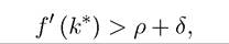
so that the capital-labor ratio is lower than the level consistent with the modified golden Recall that optimal steady-state capital-labor ratio of the neoclassical growth model satisfied the modified golden rule. In comparison, in this economy there is always underaccumulation. This contrasts with the baseline overlapping generations model, which potentially led to dynamic inefficiency and overaccumulation.

Figure 9.3 plots (9.43) and (9.49), together with the arrows indicating how average consumption per capita and capital-labor ratio change in different regions. Both (9.43) and

(9.49) are upward sloping and start at the origin. It is also straightforward to verify that while

(9.43) is concave in the k-c space, (9.49) is convex. Thus they have a unique intersection. We also know from the preceding discussion that this unique intersection is at a capital­labor ratio less than that satisfying the modified golden rule, which is marked as k_mg_r in the figure. Naturally, k_mg_r itself is less than k_gr,∣_r∣. The phase diagram also makes it clear that there exists a unique stable arm that is upward sloping in the k-c space. The shape of the stable arm is the same as in the basic neoclassical growth model. If the initial level of consumption is above this stable arm, feasibility is violated, while if it is below, the economy tends towards zero consumption and violates the transversality condition. Consequently, the steady-state equilibrium is globally saddle-path stable; consumption starts along the stable arm, and consumption and the capital-labor ratio monotonically converge to the steady state. Exercise 9.26 asks you to show local saddle-path stability by linearizing (9.43) and

(9.49) around the steady state.

The following proposition summarizes this analysis.

Proposition 9.10. In the continuous time perpetual youth model, there exists a unique steady state (k*,c*) given by (9.50) and (9.51). The level of capital-labor ratio is less than 372

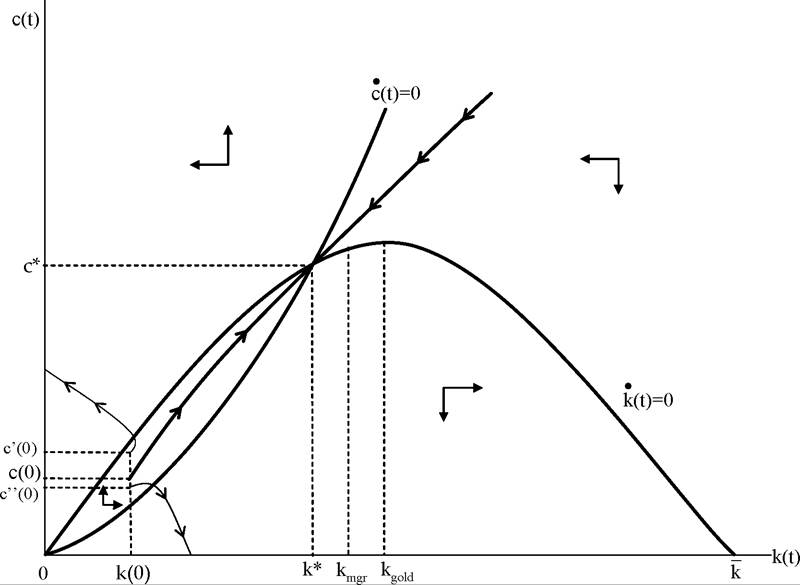
Figure 9.3. Steady state and transitional dynamics in the overlapping gen­erations model in continuous time.

the level of capital-labor ratio that satisfies the modified golden rule, k_mg_r. Starting with any k (0) > 0, equilibrium dynamics monotonically converge to this unique steady state.

Perhaps the most interesting feature of this equilibrium is that, despite finite lives and overlapping generations, there is no overaccumulation. The reason for this is that individuals have constant stream of labor income throughout their lives and thus do not need to save excessively in order to ensure smooth consumption. Is it possible to obtain overaccumulation in the continuous time perpetual youth model? The answer is yes and is demonstrated by Blanchard (1985). He assumes that each individual starts life with one unit of effective labor and then his effective labor units decline at some positive exponential rate ζ > 0 throughout his life, so that the labor earnings of an individual on generation τ at time t is exp(-ζ (t — τ)) w (t), where w (t) is the market wage per unit of effective labor at time t. Consequently, individual consumption function changes from (9.46) to

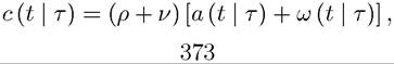
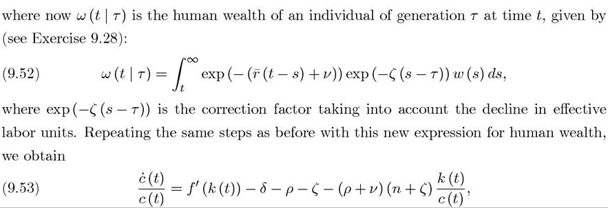
while the behavior of capital-labor ratio is still given by (9.43). It can now be shown that for ζ sufficiently large, the steady-state capital-labor ratio k* can exceed both the modified golden rule level k_mg_r and the golden rule level,(see Exercise 9.28).

This discussion therefore illustrates that overaccumulation results when there are over­lapping generations and a strong motive for saving for the future. Interestingly, it can be shown that what is important is not finite lives per se, but overlapping generations indeed. In particular, Exercise 9.30 shows that when n = 0, overaccumulation is not possible so that finite lives is not sufficient for overaccumulation. However,is possible when

n > 0 and ν = 0, so that the overlapping generations model with infinite lives can generate overaccumulation.

9.9.