Overlapping Generations with Perpetual Youth
A key feature of the baseline overlapping generation model is that individuals have finite lives and know exactly when their lives will come to an end. An alternative way of modeling finite lives is along the lines of the “Poisson death model” or the perpetual youth model introduced in Section 5.3 of Chapter 5.
Let us start with the discrete time version of that model. Recall that in that model each individual is potentially infinitely lived, but faces a probability ν ∈ (0,1) that his life will come to an end at every date (and these probabilities are independent). Recall from equation (5.9) that the expected utility of an individual with a “pure” discount factor β is given by
where u (∙) is as standard instantaneous utility function, satisfying Assumption 3, with the additional normalization that u (0) = 0. Since the probability of death is ν and is independent across periods, the expected lifetime of an individual in this model can be written as (see Exercise 9.15):

This equation captures the fact that with probability ν the individual will have a total life of length 1, with probability (1 — ν) ν, he will have a life of length 2, and so on. This model is referred to as the perpetual youth model, since even though each individual has 364
a finite expected life, all individuals who have survived up to a certain date have exactly the same expectation of further life. Therefore, individuals who survive in this economy are “perpetually young”; their age has no effect on their future longevity and has no predictive power on how many more years they will live for.
Individual i’s flow budget constraint can be written as

which is similar to the standard flow budget constraint, for example (6.40) in Chapter 6.
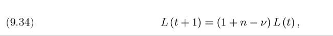
Recall that the gross rate of return on savings is 1 + r (t + 1), with the timing convention reflecting that assets at time t are rented out as capital at time t + 1. The only difference from the standard budget constraint is the additional term, Zi (t), which reflects transfers to the individual. The reason why these transfers are introduced is as follows: since individuals face an uncertain time of death, there may be “accidental bequests”. In particular, individuals will typically come to the end of their lives while their asset positions are positive. When this happens, one possibility is that the accidental bequests might be collected by the government and redistributed equally across all households in the economy. In this case, Zi (t) would represent these receipts for individual i. However, this would require that we impose a constraint of the form ai (t) ≥ 0, in order to prevent individuals from accumulating debts by the time their life comes to an end.An alternative, which avoids this additional constraint and makes the model more tractable, has been proposed and studied by Menahem Yaari and Olivier Blanchard. This alternative involves introducing life-insurance or annuity markets, where competitive life insurance firms make payments to individuals (as a function of their asset levels) in return for receiving their positive assets when they die. The term z (t) captures these annuity payments. In particular, imagine the following type of life insurance contract: a company would make a payment equal to z (a (t)) to an individual as a function of his asset holdings during every period in which he is alive.[22] [23] When the individual dies, all his assets go to the insurance company. The fact that the payment level z (a (t)) depends only on the asset holdings of the individual and not on his age is a consequence of the perpetual youth assumption— conditional expectation of further life is independent of when the individual was born and in fact, it is independent of everything else in the model. The profits of a particular insurance company contracting with an individual with asset holding equal to a (t), at time t will be With free entry, insurance companies should make zero expected profits (in terms of net present discounted value), which requires that π (a (t),t) = 0 for all t and a, thus The other important element of the model is the evolution of the demographics. Since each agent faces a probability of death equal to ν at every date, there is a natural force towards decreasing population. We assume, however, that there are also new agents who are born at every date. Differently from the basic neoclassical growth model, we assume that these new agents are not born into a dynasty; instead, they become separate households themselves. We assume that when the population at time t is L (t), there are nL (t) new households born. Consequently, the evolution of total population is given by n > v, so that there is positive population growth. Throughout this section, we ignore technological progress. An allocation in this economy is similar to an allocation in the neoclassical growth model and involves time paths for the aggregate capital stock, wage rates and rental rates of capital, notation and the life insurance contracts introduced by (9.33), the flow budget constraint of 366 an individual of generation τ can be written as: A competitive equilibrium in this economy can then be defined as follows: Definition 9.3. A competitive equilibrium consists of paths of capital stock, wage rates and rental rates of capital, - factor prices, In addition to the competitive factor prices, the key equation is the consumer Euler equation for an individual of generation τ at time t. Taking into account that the gross rate and the terms involving ν disappear. Recall that in the neoclassical model without technological progress, the consumer Euler equation admitted a simple solution because consumption had to be equal across dates for the representative household. This is no longer the case in the perpetual youth model, since different generations will have different levels of assets and may satisfy equation (9.36) with different growth rates of consumption depending on the form of the utility function u (∙). To simplify the analysis, let us now suppose that the utility function takes the logarithmic form, In that case, (9.36) simplifies to and implies that the growth rate of consumption must be equal for all generations. Using this observation, it is possible to characterize the behavior of the aggregate capital stock, though this turns out to be much simpler in continuous time. For this reason, we now turn to the continuous time version of this model (details on the discrete time model are covered in Exercise 9.22). 9.8.

 with the boundary condition L (0) = 1, where we assume that
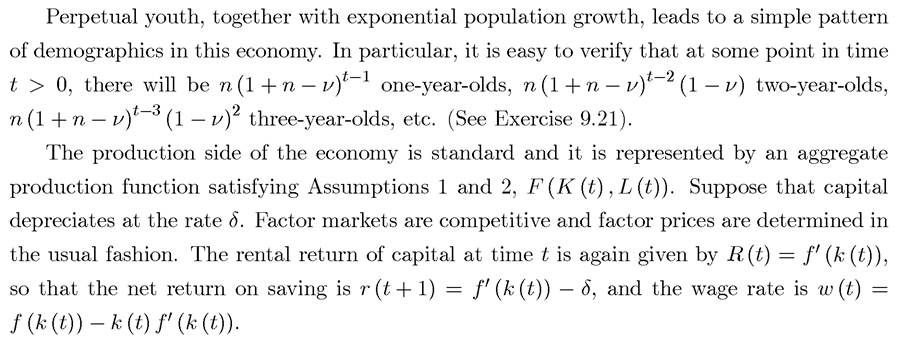
 However, it is no longer sufficient to specify aggregate consumption, since the level of consumption is not the same for all individuals. Instead, individuals born at different times will have accumulated different amounts of assets and will consume different amounts.
 Using this
 and paths of consumption for each generation,
 such that each individual maximizes utility and the time path of
  is such that given the time path of capital stock and labor
  all markets clear.
 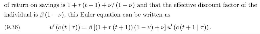 This equation looks similar to be standard consumption Euler equation, for example as in Chapter 6. It only differs from the equation there because it applies separately to each generation τ and because the term ν, the probability of death facing each individual, features in this equation. Note, however, that when both r and ν are small