Preferences, Technology and Demographics

Consider an infinite-horizon economy in continuous time. We assume that the economy admits a representative household with instantaneous utility function

(8.1)

and we make the following standard assumptions on this utility function:

ASSUMPTION 3.

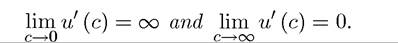
More explicitly, let us suppose that this representative household represents a set of identical households (with measure normalized to 1). Each household has an instantaneous utility function given by (8.1). Population within each household grows at the rate n, starting with L (0) = 1, so that total population is

(8.2)

All members of the household supply their labor inelastically.

Our baseline assumption is that the household is fully altruistic towards all of its future members, and always makes the allocations of consumption (among household members)

cooperatively. This implies that the objective function of each household at time t = 0, U (0), can be written as

where c (t) is consumption per capita at time t, ρ is the subjective discount rate, and the effective discount rate is ρ — n, since it is assumed that the household derives utility from the consumption per capita of its additional members in the future as well (see Exercise 8.1).

It is useful to be a little more explicit about where the objective function (8.3) is coming from.

at date t, where C (t) is total consumption and L (t) is the size of the representative household (equal to total population, since the measure of households is normalized to 1). This implies that the household will receive a utility of u (c (t)) per household member at time t, or a total utility of L (t) u (c (t)) = exp (nt) u (c (t)). Since utility at time t is discounted back to time 0 with a discount rate of exp (—ρt), we obtain the expression in (8.3).

We also assume throughout that

Assumption 4⁰.

p > n.

This assumption ensures that there is in fact discounting of future utility streams. Oth­erwise, (8.3) would have infinite value, and standard optimization techniques would not be useful in characterizing optimal plans. Assumption 4⁰ makes sure that in the model without growth, discounted utility is finite. When there is growth, we will strengthen this assumption and introduce Assumption 4.

We start with an economy without any technological progress. Factor and product mar­kets are competitive, and the production possibilities set of the economy is represented by the aggregate production function

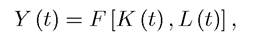
which is a simplified version of the production function (2.1) used in the Solow growth model in Chapter 2. In particular, there is now no technology term (labor-augmenting technological change will be introduced below). As in the Solow model, we impose the standard constant returns to scale and Inada assumptions embedded in Assumptions 1 and 2. The constant returns to scale feature enables us to work with the per capita production function f (∙) such 310

that, output per capita is given by

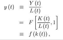
where, as before,

(8.4)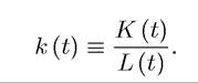

Competitive factor markets then imply that, at all points in time, the rental rate of capital and the wage rate are given by:

(8.5)

and

(8.6)

The household optimization side is more complicated, since each household will solve a continuous time optimization problem in deciding how to use their assets and allocate con­sumption over time. To prepare for this, let us denote the asset holdings of the representative household at time t by A(t).

where c (t) is consumption per capita of the household, r (t) is the risk-free market flow rate of return on assets, and w (t) L (t) is the flow of labor income earnings of the household.

Defining per capita assets as we obtain:

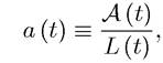
(8.7) a (t) = (r (t) — n) a (t) + w (t) — c (t).

In practice, household assets can consist of capital stock, K (t), which they rent to firms and government bonds, B (t). In models with uncertainty, households would have a portfolio choice between the capital stock of the corporate sector and riskless bonds. Government bonds play an important role in models with incomplete markets, allowing households to smooth idiosyncratic shocks. But in representative household models without government, their only use is in pricing assets (for example riskless bonds versus equity), since they have to be in zero net supply, i.e., total supply of bonds has to be B (t) = 0. Consequently, assets 311

per capita will be equal to the capital stock per capita (or the capital-labor ratio in the economy), that is,

Moreover, since there is no uncertainty here and a depreciation rate of δ, the market rate of return on assets will be given by

(8.8)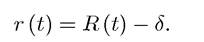

The equation (8.7) is only a flow constraint. As already noted above, it is not sufficient as a proper budget constraint on the individual (unless we impose a lower bound on assets, such as a (t) ≥ 0 for all t). To see this, let us write the single budget constraint of the form: 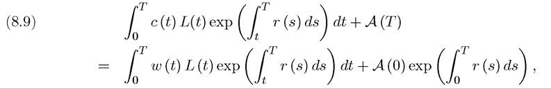for some arbitrary T > 0.

Now imagine that (8.9) applies to a finite-horizon economy ending at date T. In this case, it becomes clear that the flow budget constraint (8.7) by itself does not guarantee that A (T) ≥ 0. Therefore, in the finite-horizon, we would simply impose this lifetime budget constraint as a boundary condition.

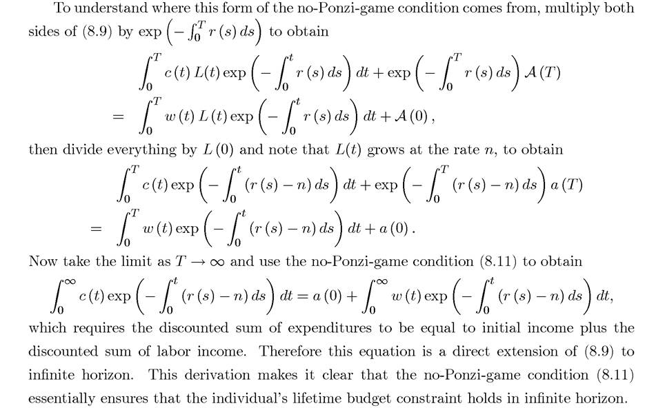
In the infinite-horizon case, we need a similar boundary condition. This is generally referred to as the no-Ponzi-game condition, and takes the form

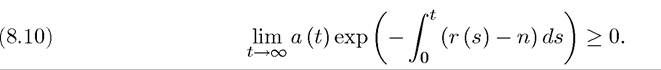
This condition is stated as an inequality, to ensure that the individual does not asymptotically tend to a negative wealth. Exercise 8.3 shows why this no-Ponzi-game condition is necessary. Furthermore, the transversality condition ensures that the individual would never want to have positive wealth asymptotically, so the no-Ponzi-game condition can be alternatively stated as:

In what follows we will use (8.10), and then derive (8.11) using the transversality condition explicitly.

The name no-Ponzi-game condition comes from the chain-letter or pyramid schemes, which are sometimes called Ponzi games, where an individual can continuously borrow from a competitive financial market (or more often, from unsuspecting souls that become part of 312

the chain-letter scheme) and pay his or her previous debts using current borrowings. The consequence of this scheme would be that the asset holding of the individual would tend to -∞ as time goes by, clearly violating feasibility at the economy level.

8.2.