Characterization of Equilibrium

8.2.1. Definition of Equilibrium. We are now in a position to define an equilibrium in this dynamic economy. We will provide two definitions, the first is somewhat more formal, while the second definition will be more useful in characterizing the equilibrium below.

Definition 8.1. A competitive equilibrium of the Ramsey economy consists of paths of consumption, capital stock, wage rates and rental rates of capital,

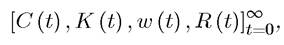such that the representative household maximizes its utility given initial capital stock K (0) and the time path of prices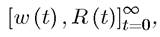and all markets clear.

Notice that in equilibrium we need to determine the entire time path of real quantities and the associated prices. This is an important point to bear in mind. In dynamic models whenever we talk of “equilibrium”, this refers to the entire path of quantities and prices. In some models, we will focus on the steady-state equilibrium, but equilibrium always refers to the entire path.

Since everything can be equivalently defined in terms of per capita variables, we can state an alternative and more convenient definition of equilibrium:

Definition 8.2. A competitive equilibrium of the Ramsey economy consists of paths of per capita consumption, capital-labor ratio, wage rates and rental rates of capital, 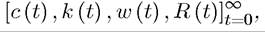such that the representative household maximizes (8.3) subject to (87) and (8.10) given initial capital-labor ratio k (0), factor prices [w (t)as in

(8.5) and (8.6), and the rate of return on assets r (t) given by (8.8).

8.2.2. Household Maximization. Let us start with the problem of the representative household. From the definition of equilibrium we know that this is to maximize (8.3) subject to (8.7) and (8.11). Let us first ignore (8.11) and set up the current-value Hamiltonian: with state variable a, control variable c and current-value costate variable μ. This problem is closely related to the intertemporal utility maximization examples studied in the previous two chapters, with the main difference being that the rate of return on assets is also time varying. It can be verified that this problem satisfies all the assumptions of Theorem 7.14, including weak monotonicity.

Thus applying Theorem 7.14, we obtain the following necessary conditions:

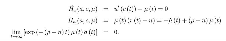
and the transition equation (8.7).

Notice that the transversality condition is written in terms of the current-value costate variable, which is more convenient given the rest of the necessary conditions.

Moreover, as discussed in the previous chapter, for any μ (t) > 0, // (a, c, μ) is a concave function of (a, c). The first necessary condition (and equation (8.13) below), in turn, imply that μ (t) > 0 for all t. Therefore, Theorem 7.15 implies that these conditions are sufficient for a solution.

We can next rearrange the second condition to obtain:

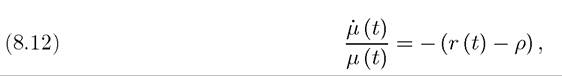
which states that the multiplier changes depending on whether the rate of return on assets is currently greater than or less than the discount rate of the household.

Next, the first necessary condition above implies that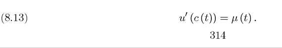

To make more progress, let us differentiate this with respect to time and divide by μ (t), which yields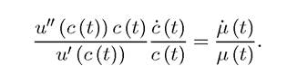

Substituting this into (8.12), we obtain another form of the famous consumer Euler equation: 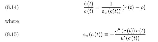is the elasticity of the marginal utility u' (c(t)).

Notice that ε_u (c (t)) is not only the elasticity of marginal utility, but even more impor­tantly, it is the inverse of the intertemporal elasticity of substitution, which plays a crucial role in most macro models. The intertemporal elasticity of substitution regulates the willingness of individuals to substitute consumption (or labor or any other attribute that yields utility) over time. The elasticity between the dates t and s > t is defined as

As s 11, we have

This is not surprising, since the concavity of the utility function u (∙)—or equivalently, the elasticity of marginal utility—determines how willing individuals are to substitute consump­tion over time.

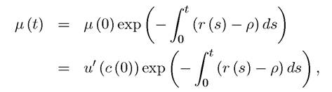
Next, integrating (8.12), we have

315

where the second line uses the first optimality condition of the current-value Hamiltonian at time t = 0. Now substituting into the transversality condition, we have

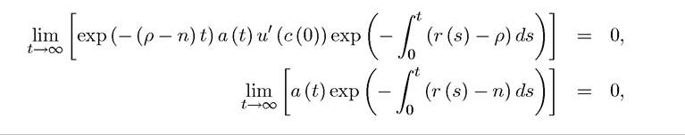
which implies that the strict no-Ponzi condition, (8.11) has to hold.

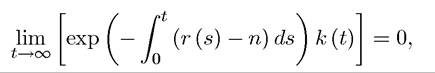
which requires that the discounted market value of the capital stock in the very far future is equal to 0. This “market value” version of the transversality condition is sometimes more convenient to work with.

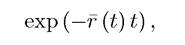
We can derive further results on the consumption behavior of households. In particular, notice that the term exp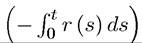is a present-value factor that converts a unit of income

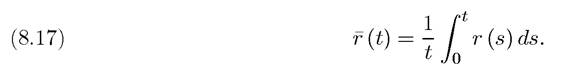
at time t to a unit of income at time 0. In the special case where r (s) = r, this factor would be exactly equal to exp(-rt). But more generally, we can define an average interest rate between dates 0 and t as

In that case, we can express the conversion factor between dates 0 and t as

and the transversality condition can be written as

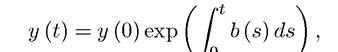
Now recalling that the solution to the differential equation

is

∖∙√ 0 /

we can integrate (8.14), to obtain

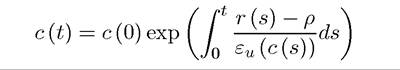
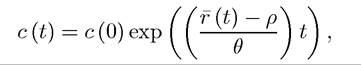
as the consumption function. Once we determine c (0), the initial level of consumption, the path of consumption can be exactly solved out. In the special case where ε_u (c (s)) is constant, 316

for example,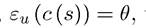this equation simplifies to

and moreover, the lifetime budget constraint simplifies to

id="Picutre 951" class="lazyload" data-src="/files/uch_group77/uch_pgroup317/uch_uch7364/image/image949.jpg">

and substituting for c (t) into this lifetime budget constraint in this iso-elastic case, we obtain 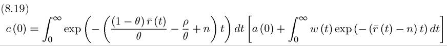as the initial value of consumption.

8.2.3. Equilibrium Prices. Equilibrium prices are straightforward and are given by

(8.5) and (8.6). This implies that the market rate of return for consumers, r (t), is given by (8.8), i.e.,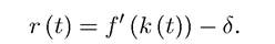

Substituting this into the consumer’s problem, we have

as the equilibrium version of the consumption growth equation, (8.14). Equation (8.19) similarly generalizes for the case of iso-elastic utility function.

8.3.