The Brock-Mirman Model

The first systematic analysis of economic growth with stochastic shocks was undertaken by Brock and Mirman in their 1972 paper. Brock and Mirman focused on the optimal growth 646

problem and solved for the social planner’s maximization problem in a dynamic neoclassical environment with uncertainty.

The economy is similar to the baseline neoclassical growth model of Chapter 8, except that the production technology is now given by

where z (t) denotes a stochastic aggregate productivity term affecting how productive a given combination of capital and labor will be in producing the unique final good of the economy. Let us suppose that z (t) follows a monotone Markov chain (as defined in Assumption 16.6) with values in the setMany applications of the neoclassical growth model

under uncertainty also assume that the stochastic shock is a labor-augmenting productivity term, so that the aggregate production function takes the form

though for the analysis here, we do not need to impose this additional restriction. Throughout we assume that the production function F satisfies Assumptions 1 and 2, and define per capita output and the per capita production function as

withonce again corresponding to the capital-labor ratio.

the existing capital stock depreciates at each date. Finally, we also suppose that the numbers zi,...,zn are arranged in ascending order and thatfor all

This assumption implies that higher values of the stochastic shock z correspond to greater productivity at all capital-labor ratios.

On the preference side, the economy admits a representative household with instantaneous utility function u (c) that satisfies the standard assumptions laid out in Assumption 3. The representative household supplies one unit of labor inelastically, so that K (t) and k (t) can be used interchangeably (and there is no reason to distinguish total consumption C (t) from per capita consumption c (t)). Finally, consumption and saving decisions at time t are made after observing the realization of the stochastic shock for time t, z (t).

The sequence version of the expected utility maximization problem of a social planner in this economy can be written as

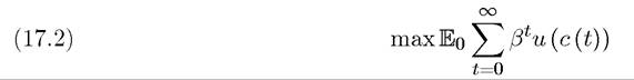
647

subject to

with given k (0) > 0. To characterize the optimal growth path using the sequence problem we would need to define feasible plans, in particular, the mappingsandintroduced in the previous chapter, withagain standing for the history of (aggregate)

shocks up to date t. Rather than going through these steps again, let us directly look at the recursive version of this program, which can be written as

The main theorems from the previous chapter immediately apply to this problem and yield the following result:

Proposition 17.1.

Proof. The proof simply involves verifying that Assumptions 16.1-16.6 from the previous chapter are satisfied, so that Theorems 16.1-16.7 can be applied. To do this, first define k such thatand show that starting with k (0) ∈ (0,k), the capital-labor

ratio will always remain within the compact set (0,^k). ?

In addition, we have:

Proposition 17.2. In the stochastic optimal growth problem described above, the policy function for next period’s capital stock, π (k,z), is strictly increasing in both of its arguments.

Proof. From Assumption 3 u is differentiable and from Proposition 17.1 V is differen­tiable in k. Moreover, by the same argument as in the proof of Proposition 17.1, k ∈ (0, ^k), thus we are in the interior of the domain of the objective function. Thus, the value function V is differentiable in its first argument and we have

where V⁰ denotes the derivative of the V (k,z) function with respect to its first argument. Since from Proposition 17.1 V is strictly concave in k, this equation can hold when the level of k or z increases only if k⁰ also increases. For example, an increase in k reduces the first-term (because u is strictly concave), hence an increase in k⁰ is necessary to increase the first term and to reduce the second term (by the concavity of V). The argument for the implications of an increase in z is similar.

It is also straightforward to derive the stochastic Euler equations corresponding to the neoclassical growth model with uncertainty. For this purpose, let us first define the policy function for consumption as

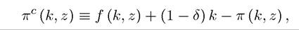
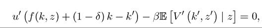
where π (k, z) is the optimal policy function for next date’s capital stock determined in Proposition 17.1. Using this notation, the stochastic Euler equation can be written as

where f⁰ denotes the derivative of the per capita production function with respect to the capital-labor ratio, k. In this form, the Euler equation looks complicated. A slightly different way of expressing this equation makes it both simpler and more intuitive:

wheredenotes the expectation conditional on information available at time t and p (t + 1) is the stochastic marginal product of capital (including undepreciated capital) at date t + 1. This form of writing the stochastic Euler equation is also useful for comparison with the competitive equilibrium because p (t + 1) corresponds to the stochastic (date t + 1) dividends paid out by one unit of capital invested at time t.

Although Proposition 17.1 characterizes the form of the value function and policy func­tions, it has two shortcomings. First, it does not provide us with an analog of the “Turnpike Theorem” of the non-stochastic neoclassical growth model. In particular, it does not char­acterize the long-run behavior of the neoclassical growth model under uncertainty. Second, while the characterization provides a number of qualitative results about the value and the policy functions, it does not deliver comparative static results.

A full analysis of the long run behavior of the stochastic growth model would take us too far afield into the analysis of Markov processes. Nevertheless, a few simple observations are useful to appreciate the salient features of the stochastic law of motion of the capital-labor ratio in this model. The capital stock at date t +1 is given by the policy function π, thus we have

which defines a general Markov process, since before the realization of z (t), k (t + 1) is a random variable, with its law of motion governed by the last period’s value of k (t) and the realization of z (t). If z (t) has a non-degenerate distribution, k (t) does not typically converge to a single value (see Exercise 17.4). Instead, we may hope that it will converge to an invariant limiting distribution. It can indeed be verified that this is the case. The Markov process (17.7) defines a sufficiently well-behaved stochastic process that starting with any k (0), it converges to a unique invariant limiting distribution, meaning that when we look at sufficiently faraway 649

horizons, the distribution of k should be independent of k (0). Moreover, the average value of k (t) in this invariant limiting distribution will be the same as the time average of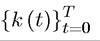 as T → ∞ (so that the stochastic process for the capital stock is “ergodic”). Consequently, a “steady-state” equilibrium now corresponds not to specific values of the capital-labor ratio and output per capita but to invariant limiting distributions. If the stochastic variable z (t) takes values within a sufficiently small set, this limiting invariant distribution would hover around some particular values, which we may wish to refer to as “quasi-steady-state” values of the capital-labor ratio, because even though the equilibrium capital-labor ratio may not converge to this value, it will have a tendency to return to a neighborhood thereof.

To obtain a better understanding of the behavior of the neoclassical growth model under uncertainty, we next consider a simple example, which allows us to obtain a closed-form solution for the policy function π.

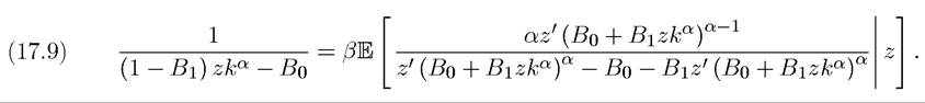
Example 17.1. Suppose that u (c) = log c, F (K, L, z) = zK^αL^1-α, and δ = 1. We continue to assume that z follows a Markov chain over the set Z ? {zχ,...,z^}, with transition probabilities denoted by Qjj'. Let k ? K/L. The stochastic Euler equation (17.5) implies 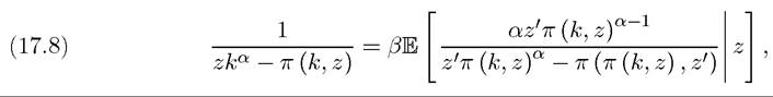which is a relatively simple functional equation in a single function π (∙, ∙). Though simple, this functional equation would still be difficult to solve unless we had some idea about what the solution looked like. Here, fortunately, the method of “guessing and verifying” the solution of the functional equation becomes handy. Let us conjecture that

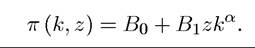
Substituting this guess into (17.8), we obtain

It is straightforward to check that this equation cannot be satisfied for any) (see Exercise 17.5). Thus imposing Bo = 0 and writing out the expectation explicitly with this expression becomes

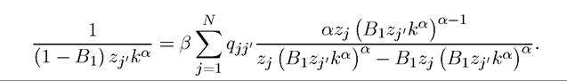
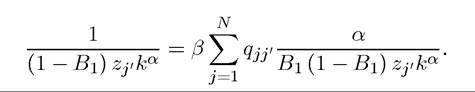
Simplifying each term within the summation, we obtain

650

Now taking Zji and k out of the summation and using the fact that, by definition, ∣ qjj' =

1, we can cancel the remaining terms and obtain

so that irrespective of the exact Markov chain for z, the optimal policy rule is

The reader can verify that this is identical to the result in Example 6.4 in Chapter 6, with z there corresponding to a non-stochastic productivity term. Consequently, in this case the stochastic elements have not changed the form of the optimal policy function. Exercise 17.6 shows that the same result applies when z follows a general Markov process rather than a Markov chain.

Using this example, we can fully analyze the stochastic behavior of the capital-labor ratio and output per capita. In fact, the stochastic behavior of the capital-labor ratio in this economy is identical to that of the overlapping generations model analyzed in Section 17.5 and Figure 17.1 in that section applies exactly to this example. A more detailed discussion of these issues is left to Exercise 17.7. Unfortunately, Example 17.1 is one of the few instances of the neoclassical growth model that admit closed-form solutions. In particular, if the depreciation rate of the capital stock δ is not equal to 1, the neoclassical growth model under uncertainty does not admit an explicit form characterization (see Exercise 17.8).

17.2.