Equilibrium Growth under Uncertainty

Let us now consider the competitive equilibria of the neoclassical growth model under uncertainty. The environment is identical to that in the previous section and z corresponds to an aggregate productivity shock affecting all production units and all households.

Here I will briefly discuss the explicit characterization of competitive equilibria of this economy both to show the equivalence between the optimal growth problem and the equilib­rium growth problem under complete markets and also to introduce a number of important 651

ideas related to the pricing of various contingent claims in competitive equilibrium under uncertainty. The reference to complete markets in this context implies that, in principle, any commodity, including any contingent claim, can be traded competitively. Nevertheless, as shown by our analysis in Section 5.8 in Chapter 5, in practice there is no need to specify or trade all of these commodities and a subset of the available commodities is sufficient to provide all the necessary trading opportunities to households and firms.

Preferences and technology are as in the previous section. Recall that the economy admits a representative household and that the production side of the economy can be represented by a representative firm (Theorem 5.4). Let us first consider the problem of the representative household. This household will maximize the objective function given by (17.2) subject to the lifetime budget constraint (written from the viewpoint of time t = 0). The analysis in Section 5.8 in Chapter 5 shows that there is no loss of generality in considering the competitive equilibrium from the viewpoint of time t = 0 relative to formulating it with sequential trading constraints. It is nonetheless useful to spell out this equivalence by showing how the baseline neoclassical growth model under uncertainty can be analyzed both assuming that all trades take place at date t = 0 and also under sequential trading.

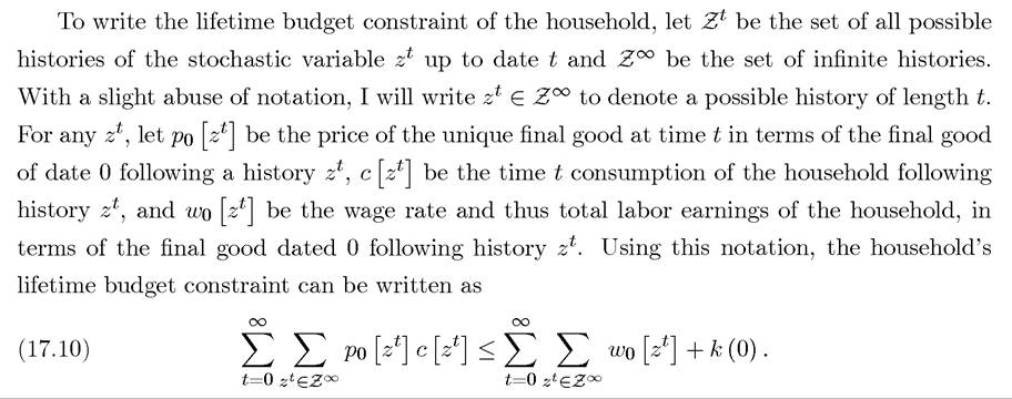
A number of features about this lifetime budget constraint are worth noting.¹ First, there are no expectations. This is because we are considering an economy with complete markets, which implies that the household is making all of his (lifetime) trades in the initial period of the economy t = 0 at a well-defined price vector for all Arrow-Debreu commodities. Consequently, the lifetime budget constraint applies in exactly the same way as a static budget constraint

652

in the standard theory of general equilibrium. More explicitly, the household buys claims to different “contingent” consumption bundles. These bundles are contingent in the sense that they are conditioned on the history of the aggregate state variable (stochastic shock) z^t and thus whether they are realized and delivered depends on the realization of the sequence of the stochastic shock.

at time t if history z^t is realized. If a different history is realized, then this claim will not be realized. This way of writing the lifetime budget constraint reiterates the importance of thinking in terms of Arrow-Debreu commodities.

Second, with this interpretation the left-hand side is simply the total expenditure of the individual taking the prices of all possible claims, i.e., the entire set of, as given. The right-hand side has a similar interpretation, except that it denotes the labor earnings of the household rather than his expenditures. The last term on the right-hand side is the value of the initial capital stock per capita, which is part of the household’s initial wealth. As noted above, the price of the final good at date t = 0 is normalized to 1. As in the standard neoclassical growth model, capital is in terms of the final good, thus has a price of 1 as well.^[36]

Finally, the right-hand side of (17.10) could also include profits accruing to the individuals (as in Definition 5.1 in Chapter 5). The fact that the aggregate production function exhibits constant returns to scale combined with the presence of competitive markets implies that equilibrium profits will be equal to 0. This enables us to omit the additional term referring to profits in the representative household’s budget constraint without loss of any generality.

The objective function of the household at time t = 0 can also be written somewhat more explicitly than (17.2) as follows:

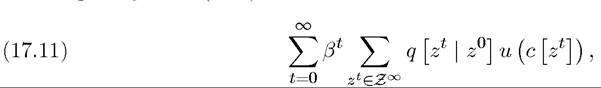
where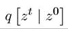is the probability at time 0 that the history z^t will be realized at time t.

have written this in the form of a conditional probability to create continuity between the treatment based on trades at date t = 0 and sequential trading. Notice that there is no longer the expectations operator in this objective function because the explicit summation over all possible events weighted by their probabilities has been introduced instead.

Although we will shortly formulate the problem of the representative household recur­sively, we can already understand the structure of the equilibrium by looking at the sequence problem of maximizing (17.11) subject to (17.10). Assuming that the interior solution exists,

the first-order conditions of this problem is

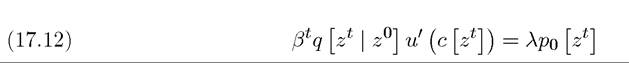
for all t and all z^t, where λ is the Lagrange multiplier on (17.10) and now does in fact correspond to the marginal utility of income at date t = 0 (see Exercise 17.11 on why a single multiplier for the lifetime budget constraint is sufficient in this case). Combining this first-order condition for two different date t histories z^t and z^t, we obtain

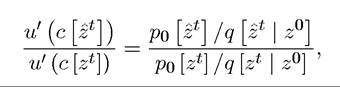
which shows that the right-hand side is the relative price of consumption claims conditional on histories z^t and z^t. Combining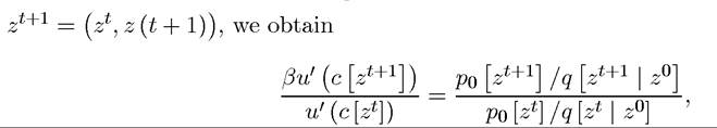this first-order condition for histories z^t and z^t+1 such that so that the right-hand side now corresponds to the contingent interest rate between date t and t + 1 conditional on z^t (and contingent on the realization ofWhile these expressions are intuitive, they cannot be used to characterize equilibrium consumption or investment sequences until we know more about the prices poWe will be able to derive these prices

from the profit maximization problem of the representative firm.

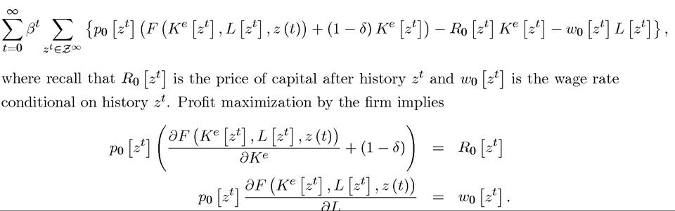
Let us consider the value of the firm at date t = 0. To do this, let us de fine one more price sequence, Ro [z^l/ corresponding to the price of one unit of capital after the state has been revealed as z^t and also denote the capital and labor employment levels of the representative firm after history z^t byandNotice that I have introduced the additional superscript “e” for the capital to distinguish the capital employed by the firm after history z^t from the capital that is saved by the households after history z^t. These two objects are quite different as we will see.

The value of the firm can then be written as

654

Using constant returns to scale and expressing everything in per capita terms, these first-order conditions can be written as

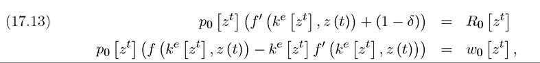
where f' denotes the derivative of the per capita production function with respect to the capital-labor ratioThe first equation relates the price of the final good to the

price of capital goods and to the marginal productivity of capital, while the second equation determines the wage rate in terms of the price of the final good and the marginal (physical) product of labor. Equation (17.13) can also be interpreted as stating that the price of a unit of capital good after history z^t, Ro [z^t~^, is equal to the value of dividends paid out by this unit of capital inclusive of undepreciated capital, that is, the price of the final good, pθ [z^t), times the marginal product of capitalplus the (1 — δ) fraction of the capital that

is not depreciated and paid back to the holder of the capital good in terms of date t +1 final good.

To complete the characterization of a competitive equilibrium, we need to impose market clearing. For labor, this is straightforward and requires

To write the market clearing condition for capital, recall that per capita production after his- because the amount of available capital at time t is fixed irrespective of the realization of z (t + 1). The capital market clearing condition can then be written as

655

which is identical to (17.6). Given this first-order condition, it is straightforward to prove the equivalence between the optimal growth path and the competitive growth path (in this instance using the sequence approach).

Proposition 17.3. In the above-described economy, optimal and competitive growth path coincide.

Proof. See Exercise 17.13. ?

Complementary insights can be obtained by considering the equilibrium problem in its equivalent form with sequential trading rather than all trades taking place at the initial date t = 0. To do this, we will write the budget constraint of the representative household somewhat differently. First, normalize the price of the final good at each date to 1 (recall the discussion in Section 5.8 in Chapter 5). The a [z^l'] s now correspond to Basic Arrow securities that pay out only in specific states on nature. More explicitly, a [z^l'] denotes the assets of the household in terms of the final good at date t conditional on history z^t. We interpret as a set of contingent claims that the household has purchased that will pay a z^t units of the final good at date t when history z^t is realized. We also denote the price of claim to one unit of a [z) at time t — 1 after history z^t-1 by, where naturally

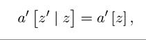
z^t = (z^t-1,z (t)). The amount of these claims purchased by the household is denoted by a [(z^t-1,z (t)}]. Consequently, the flow budget constraint of the household can be written as 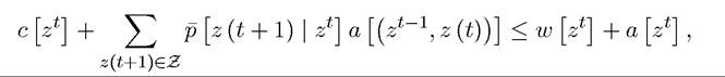where w [z^l'] is the equilibrium wage rate after history z^t in terms of final goods dated t, so the right-hand side is the total amount the resources available to the household after directly go to the recursive formulation, leaving the sequence version of the household’s problem with sequential trading to Exercise 17.14.

Preparing for the recursive formulation, let a denote the current asset holdings of the household (in terms of the notation above, you can think of this as the realization of the current assets after some history z^t has been realized). Then the flow budget constraint of the household can be written as

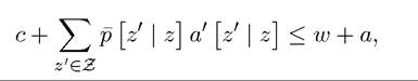
where the functionsummarizes the prices of contingent claims (for next date’s state z⁰ given current state z) anddenotes the corresponding asset holdings. Let V (a, z) be the value function of the household when it holds a units of the final good as assets and the current realization of the stochastic variable is z. The choice variables of the household are contingent asset holdings for the next date, denoted byand consumption today denoted by c [a, z]. Let us also denote the probability that next period’s stochastic variable will be equal to z⁰ conditional on today’s value being z byThen taking the sequence 657

of equilibrium prices p as given, the value function of the representative household can be written as

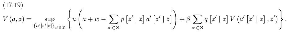
Theorems 16.1-16.7 from the previous chapter can again be applied to this value function (see Exercise 17.15). The first-order condition for current consumption can now be written asid="Picutre 2237" class="lazyload" data-src="/files/uch_group77/uch_pgroup317/uch_uch7364/image/image2235.jpg">

for any z' ∈ Z with c [a, z] denoting the optimal consumption conditional on asset holdings a and stochastic variable z. Since this equation refers to the representative household and asset holdings, in the form of capital, are decided before next period’s stochastic shock z⁰ is realized, the capital market clearing condition once again requires

so that, in the aggregate, the same amount of assets will be present in all states at the next date. This implies that the first-order condition for consumption can be alternatively written as

With a similar reasoning to before, the no arbitrage condition implies

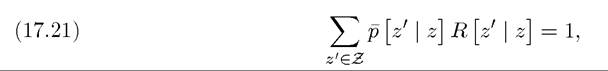
where R [z⁰ | z] is the price of capital goods when the current state is z⁰ and last period’s state was z. Intuitively, the cost of one unit of the final good now, which is 1, has to be equal to the return that the individual will obtain by carrying this good to the next period and selling it as a capital good then. When tomorrow’s state is z⁰, the gross rate of return in terms of tomorrow’s goods is R [z⁰ | z] and the relative price of tomorrow’s goods in terms of today’s goods is p [z⁰ | z]. Summing over all possible states z⁰ tomorrow must then have total return of 1 to ensure no arbitrage (see Exercise 17.16). Let us now combine (17.20) with the envelope condition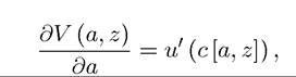

and then multiply both sides of (17.20) by R [z⁰ | z] and sum over all z⁰ ∈ Z to obtain the first-order condition of the household as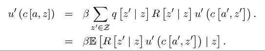

Next the market clearing condition for capital, combined with the fact that the only asset in the economy is capital, implies that

Therefore, this first-order condition can be written as

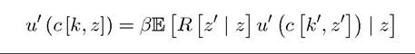
which is identical to (17.6). This again shows the equivalence between the social planner’s problem and the competitive equilibrium path.

Given the equivalence between the social planner’s problem (the optimal growth problem) and the characterization of the equilibrium and the fact that the former is considerably simpler, much of the literature focuses on the social planner’s problem when this can be done. The social planner’s problem characterizes the equilibrium path of all the real variables and the comparison of the analysis in this section to that in the previous section shows that various different prices are also straightforward to obtain from the Lagrange multiplier of the social planner’s problem. Here the most important prices are those for capital goods, i.e., the R [z' | z]s. Equations (17.5) and (17.6) show that these can be easily obtained from the marginal product of capital in the optimal growth path.

17.3.