Application: Real Business Cycle Models
One of the most important applications of the neoclassical growth model under uncertainty over the past 25 years has been to the analysis of short- and medium-run fluctuations. The approach, pioneered by Kydland and Prescott’s seminal (1982) paper and referred to as the Real Business Cycle theory, uses the neoclassical growth model with aggregate productivity shocks in order to provide a framework for the analysis of macroeconomic fluctuations.
The Real Business Cycle (RBC) theory has been one of the most active research areas of macroeconomics in the 1990s and also one of the most controversial. On the one hand, its conceptual simplicity and its relative success in matching certain moments of employment, consumption and investment fluctuations for a given (appropriately chosen) sequence of aggregate productivity shocks have attracted a large following. On the other and, the absence of monetary factors and demand shocks, the traditional pillars of Keynesian economics and previous research on macroeconomic fluctuations, has generated a ferocious opposition and much debate on the merits of this theory. The merits of the RBC theory are not relevant for our focus here and would take us too far afield from the key questions of economic growth. Nevertheless, a brief exposition of the canonical RBC model is useful for two purposes. First, it constitutes one of the most important applications of the neoclassical growth model under uncertainty and has become another one of the workhorse models for macroeconomic research over the past 25 years. Second, it illustrates how the introduction of labor supply 659choices into the neoclassical growth model under uncertainty generates new insights. So far I have assumed, except in Exercise 8.17 in Chapter 8, that labor is supplied inelastically and this choice has enabled us to focus on the first-order issues related to economic growth.
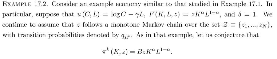
Because the issue of labor supply is central to a number of questions in macroeconomics, a brief analysis of the neoclassical growth model with labor supply is also useful.The economic environment is identical to that in the previous two sections, with the only difference that the instantaneous utility function of the representative household now takes the form
where C denotes consumption and L labor supply. I use uppercase letters for consistency with what will come below. I assume that u is jointly concave and continuously differentiable in both of its arguments and strictly increasing in C and strictly decreasing in L. I also assume that L has to lie in some convex compact set [0, L].
Given the equivalence between the optimal growth and the equilibrium growth problems, I will focus on the optimal growth formulation here and set up the social planner’s problem. This problem can be expressed as the maximization of
subject to the flow resource constraint

where z (t) again represents an aggregate productivity shock following a monotone Markov chain.
The social planner’s problem can be written recursively as
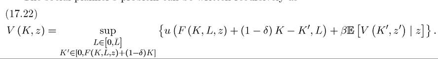
The following proposition is again a direct consequence of Theorems 16.1-16.7:
Proposition 17.4. The value function V (K,z) defined in (17.22) is continuous and strictly concave in K, strictly increasing in K and z, and differentiable in K > 0. There exist uniquely defined policy functions hat determine the level of
capital stock chosen for next period and the level of labor supply as a function of the current capital stock K and the stochastic variable z.
Proof. See Exercise 17.17. ?
Clearly, once again assuming an interior solution, the relevant prices can be obtained from the appropriate multipliers and the standard first-order conditions characterize the form of 660
the equilibrium. In particular, the two key first-order conditions determine the evolution of consumption over time and the equilibrium level of labor supply. Denoting the derivatives of the u function with respect to its first and second arguments by uc and u∣ι, the derivatives of the F function by Fk and Fi, and defining the policy function for consumption as  these take the form
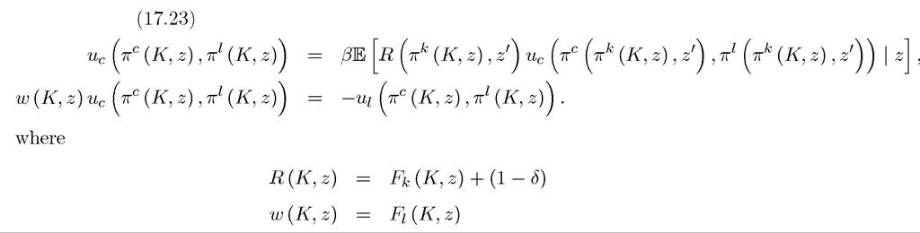
denote the gross rate of return to capital and the equilibrium wage rate. Notice that the first condition in (17.23) is essentially identical to (17.5), whereas the second is a static condition determining the level of equilibrium (or optimal) labor supply. The second condition does not feature expectations, since it is conditional on the current value of the capital stock, K, and the current realization of the aggregate productivity variable, z.
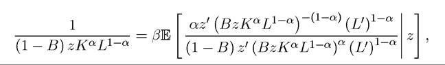
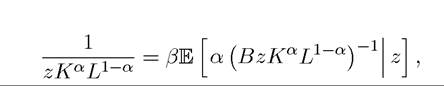
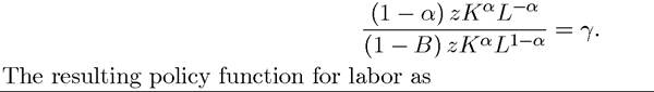
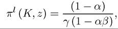
Why is this framework useful for the analysis of macroeconomic fluctuations? The answer lies in the fact that estimates of total factor productivity, along the lines described in Chapter 3, indicate that it is procyclical—that is, it is higher in periods during which output is above trend and unemployment is low. So let us think of a period in which z is low. Clearly, if there is no offsetting change in labor supply, output will be low, so we can think of this period as a “recession”. Moreover, under standard assumptions, the wage rate w (K,z) and equilibrium labor supply will decline.[37] [38] Thus there will be low employment as well as low output. Thus a negative productivity shock generates two of the important characteristics of a recessionary period. In addition, if the Markov chain (or more generally the Markov process) governing the behavior of z exhibits persistence, output will be low the following period as well, so output and employment will exhibit persistent fluctuations. Finally, provided that the aggregate production function F (K, L, z) takes a form such that low output is also associated with low marginal product of capital, the expectation of future low output will typically reduce savings and thus future levels of capital stock (though this does also depend on the form of the utility function, which regulates the desire for consumption smoothing and the balance between income and substitution effects). This brief discussion suggests that the neoclassical growth model under uncertainty with labor supply choices and with aggregate productivity shocks may generate some of the major qualitative features of macroeconomic fluctuations. The RBC literature also argues that this model, under suitable assumptions, generates the major quantitative features of the business cycles, such as the correlations between output, investment, and employment. A large part of the debate on the merits of the RBC model focused on: (i) whether the model did indeed match these moments in the data; (ii) whether these were the right empirical objects to look at (for example, as opposed to persistence in employment or output at different frequencies); and (iii) whether a framework in which the driving force of fluctuations is exogenous changes in aggregate productivity is sidestepping the more interesting question of why there are shocks that cause recessions and booms. It is fair to say that, while the RBC debate is not as active today as it was in the 1990s, there has not been a complete agreement on these questions. In the meantime, many extensions of the standard RBC model have improved over the bare-bones version presented here. The model presented here considered the neoclassical growth model without exogenous technological progress. Then with these functional forms, the stochastic Euler equation for consumption (17.23) implies where L' denotes next period’s labor supply. Canceling constants within the expectations and taking terms that do not involve z' out of the expectations operator this equation simplifies to which yields which is identical to that in Example 17.1. Next, considering the first-order condition for labor, we obtain which implies that labor supply is constant. This is because with the preferences as specified here, the income and the substitution effects cancel out, thus the increase in wages induced by a change in aggregate productivity has no effect on labor supply. Exercise 17.19 shows that the same result obtains whenever the utility function takes the form of U (C, B) = log C+h (L) for some decreasing and concave function h. Overall, this simple version of the RBC model with a closed-form solution therefore replicates the covariation in output and investment, but does not generate labor fluctuations. 17.4.