Growth with Incomplete Markets: The Bewley Model

We now turn to a fundamentally different model of economic growth, where the econ­omy does not admit a representative household and idiosyncratic risks are not diversified. This model was first introduced and studied by Truman Bewley (1977, 1980, 1986).

The economy is populated by a continuum 1 of households and the set of households is denoted by H. Each household has preferences given by (17.2) and supplies labor inelastically. Suppose also that the second derivative of this utility function, u" (∙), is increasing. Differently from the baseline neoclassical growth model, the efficiency units that each household supplies 663

vary over time. In particular, each household h ∈ H has a labor endowment of z^h (t) at time t, where z^h (t) is an independent draw from the set Z ? [z_mi_n,z_max], where 0 < '_j∣∣_i∣∣ < z_max < ∞, so that the minimum labor endowment is z_mi_n.

The production side of the economy is the same as in the canonical neoclassical growth model under certainty and is represented by an aggregate production function satisfying Assumptions 1 and 2, as in (17.1). The only difference is that L (t) is now the sum (integral) of the heterogeneous labor endowments of all the agents and is written as

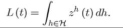
Appealing to a law of large numbers type argument, we assume that L (t) is constant at each date and we normalize it to 1. Thus output per capita in the economy can be expressed as

with k (t) = K (t). Notice that there is no longer any aggregate productivity shock. The only source of uncertainty is at the individual level (i.e., it is idiosyncratic). Consequently, while individual households will experience fluctuations in their labor income and consump­tion, we can imagine a stationary equilibrium in which aggregates are constant over time. Throughout this section I focus on such a stationary equilibrium. In particular, in a station­ary equilibrium the wage rate w and the gross rate of return on capital R will be constant (though of course their levels will be determined endogenously to ensure equilibrium). Let us first take these prices as given and look at the behavior of a typical household h ∈ H (I am using the language “typical” household, since, though not representative, this household faces an identical problem to all other households in the economy). This household will solve the following maximization problem: maximize (17.2) subject to the flow budget constraint

for all t, where α^h (t) is the asset holding of household h ∈ H at time t.

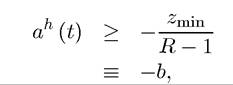
for all t. We can then write the maximization problem of household h ∈ H recursively as

Standard dynamic programming arguments then establish the following proposition:

Proposition 17.5. The value function V^h (a, z) defined in (17.2f) is uniquely defined, continuous and strictly concave in a, strictly increasing in a and z, and differentiable in a ∈ (-b, Ra + wz). Moreover, the policy function that determines next period’s asset holding π (a, z) is uniquely defined and continuous in a.

Proof. See Exercise 17.20.

Moreover, as in Proposition 17.2, we have the additional result on the form of the policy function:

Proposition 17.6. The policy function π (a,z) derived in Proposition 17.5 is strictly increasing in a and z.

Proof. See Exercise 17.21.

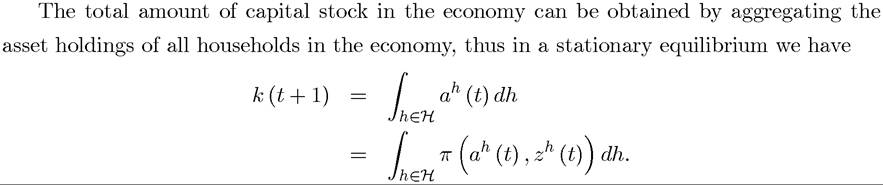
This equation integrates over all households taking their asset holdings and the realization of their stochastic shock as given. It states that both the average of current asset holdings and also the average of tomorrow’s asset holdings must be equal by the definition of a stationary equilibrium. To understand this condition, recall that as in the neoclassical growth model, the policy function a⁰ = π (a, z) defines a general Markov process. Under fairly weak assumptions this Markov process will admit a unique invariant distribution.

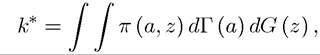
which uses the fact that z is distributed identically and independently across households and over time.

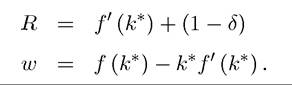
Next turning to the production side, we have the same factor prices as the neoclassical growth model under certainty, i.e.,

Recall from Chapters 6 and 8 that the neoclassical growth model with complete markets and no uncertainty implies that there exists a unique steady state in which βR = 1, i.e.,

where k** refers to the capital-labor ratio of the neoclassical growth model under certainty.

Perhaps the most interesting implication of the Bewley economy is that this is no longer true. In particular, we have

Proposition 17.7. In any stationary equilibrium of the Bewley economy, we have that the stationary equilibrium capital-labor ratio k* is such that and

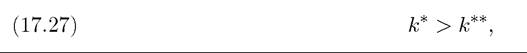
where k** is the capital-labor ratio of the neoclassical growth model under certainty.

Proof. (Sketch) Suppose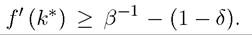Then the result in Exercise 16.10

from the previous chapter implies that each household’s expected consumption is strictly increasing. This implies that average consumption in the population, which is deterministic, is strictly increasing and would tend to infinity.

Intuitively, the interest rate in the incomplete markets economy is “depressed” relative to the neoclassical growth model with certainty because each household has an additional self-insurance (or precautionary) incentive to save. These additional savings increase the capital-labor ratio and reduce the equilibrium interest rate. Interestingly, therefore, the Bewley economy, like the overlapping generations model of Chapter 9, leads to a higher capital intensity of production than the standard neoclassical growth model. Observe that in both cases, the lack of a representative household plays an important role in this result.

While the Bewley model is an important workhorse for macroeconomic analysis, two features, that may be viewed as potential shortcomings, are worth noting here. First, as we already remarked in the context of the overlapping generations model, the source of 666

inefficiency coming from overaccumulation of capital is unlikely to be important for explaining income per capita differences across countries. Thus the Bewley model is not interesting because of the greater capital-labor ratio that it generates. Instead, it is important as an illustration of how an economy might exhibit a stationary equilibrium in which aggregates are constant while individual households have uncertain and fluctuating consumption and income profiles. It also emphasizes issues of individual risk in the context of a relatively familiar neoclassical growth setup. Issues of individual risk bearing are important in the context of economic development as shown in Section 17.6 below and also in Chapter 21. Second, the incomplete markets assumption in this model may be extreme. In practice, when their incomes are low, individuals do receive transfers, either because they have entered into some form of private insurance or because of government-provided social insurance. Instead, the current model exogenously assumes that there are no insurance possibilities. Much more satisfactory would be models in which the lack of insurance opportunities are derived from microfoundations (for example, from moral hazard or adverse selection) or models in which the set of active markets is determined endogenously. While models of limited insurance due to moral hazard or adverse selection are beyond the scope of this book, we will return to an economic growth model with endogenously incomplete markets in Section 17.6.

17.5.