Distributional Conflict and Economic Growth: Concave Preferences*

In this section, I provide a preliminary analysis of an environment similar to the baseline model studied so far, but with concave preferences. My main purpose is to illustrate how to approach the analysis of such an economy and highlight some of the additional conceptual and technical issues that arise in this case.

Relative to the the framework in Section 22.2 I make two different assumptions. First, preferences are now assumed to take the form

where U (∙) is a strictly increasing, strictly concave and continuously differentiable utility function. This specification assumes that all three groups have the same utility function, though this is not important for the analysis and is simply adopted to reduce notation. The second important assumption is that we close all financial markets. Consequently, entrepre­neurs cannot borrow in order to invest in capital, and have to save by reducing their current consumption. Note that in the absence of political economy (and taxes), this would have no effect on the qualitative features of the dynamics of the model, which still closely resemble those of the baseline neoclassical growth model. In particular, without any taxes, there ex­ists a unique globally (saddle-path) stable steady-state equilibrium, which satisfies equation 969

(6.38) in Chapter 6. All the other assumptions from Section 22.2, especially those regarding the production functions and the timing of policies, continue to apply.

Using exactly the same notation as in Section 22.2, the dynamic optimization of middle­class entrepreneurs for a given sequence of policies and wages, p^t and w^t, can be written as

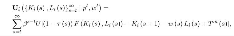
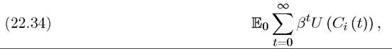
where I have set the depreciation rate of capital δ equal to 1 to simplify the notation.

the analysis so far that there will never be 100% taxation, thus we can restrict attention to such tax sequences and the maximization problem of each entrepreneur is indeed a strictly concave problem.

The relevant necessary and sufficient first-order conditions for entrepreneur i can be written as

for each t, which looks identical to the Euler equation for the representative consumer given in (6.37) in Chapter 6. This is not surprising, since each entrepreneur solves a similar program to that facing the representative consumer or the social planner in the basic neoclassical growth model. The only difference is the presence of the taxes, which implies that one unit of consumption foregone today does not earn the full marginal product of capital, but only that left over from taxes. This equation implies that the capital-labor ratio are chosen by entrepreneur i will now depend on the entire sequence of taxes, since these taxes will influence the current and future consumption levels. Consequently, we no longer have a simple equation such as (22.11) in Section 22.2. Nevertheless, (22.35) does determine a unique sequence of capital-labor ratio choices for each entrepreneur given the sequence of taxes and their initial capital stock, Ki (0).

To simplify the analysis, let us suppose that all entrepreneurs start with the same initial capital stock, i.e., Ki (0) = K (0). Given the symmetric initial conditions and the strict concavity of the problem, the equilibrium will be symmetric as well and each entrepreneur will choose exactly the same capital-labor ratio sequence.

elite to choose some p⁰ ∈ P to maximize their discounted utility. This would indeed be the solution to the political economy problem if the elite could commit to a sequence of policies at date t = 0. But the assumption we have made so far, which is a natural approximation to reality, is that political decisions are made sequentially, and commitment to a future sequence of policies is not possible. This is exactly where my treatment in the Section 22.2 cut some corners. With linear utility, it did not matter whether the elite chose the sequence of policies at date t = 0 or sequentially as specified in the timing of events. To simplify the discussion there, I did not dwell on this distinction. This distinction now becomes crucial.

The right way to approach this problem is to specify the payoff-relevant state variables and then at each date have the elite make their utility-maximizing policy choices (as a function of the payoff-relevant state variables). The major difference from the analysis in this chapter so far is that once the elite undertake a deviation the future sequence of policies should not remain fixed but also change, because the deviation will have affected the evolution of the state variables and the evolution of the state variables will induce a different set of preferred policies for the elite. With linear preferences the deviation had no effect on future equilibrium policies, thus the analysis in the previous sections did not explicitly specify the effect of a deviation on the future sequence of policies. To show how this can be done in general and what its implications will be are the main focus of this section.

Let us now start developing the notation and the language for such an analysis. Most generally, the relevant state variable at time t would be a distribution of capital stocks or capital-labor ratios across all entrepreneurs denoted byThis would significantly

complicate the analysis, since working with entire distributions as the state variable is diffi­cult. Fortunately, we can circumvent this problem. The same type of argument used above for a specific sequence of policies implies that, even taking the potential changes in future policies into account, the maximization problem of each entrepreneur is strictly concave. In addition, each entrepreneur recognizes that he has no effect on aggregates and also all entre­preneurs start with the same initial condition. Thus we can restrict attention to a situation in which at all dates all entrepreneurs will choose the same capital-labor ratio, and the state variable at time t can be represented by the capital-labor ratio of the “representative” entre­preneur,Moreover, as in Chapter 6, the Inada conditions in Assumption 2 imply

that we can restrict attention to state variables in a compact set

³It may appear that we are cutting some corners here as well. All entrepreneurs choose the same capital­labor ratio along-the-equilibrium path. What happens if an entrepreneur takes a deviation? It would appear that at that point, the state variable can no longer be represented by a one-dimensional object, and to take care of behavior off-the-equilibrium path properly, we would need to consider state variables of much higher dimension. Fortunately, this is not an issue, thanks to the fact that there is a continuum of entrepreneurs. If a single entrepreneur takes a deviation, this will have no effect on aggregates.

Given this state variable, the policy choice of the elite can be represented by a policy function denoted by

which determines the utility-maximizing tax rate for the elite at the next date, τ (t + 1), as a function of the current capital-labor ratio k (t). We could extend this function so that it also determines the amount of transfers. But this is not necessary, since, as in the previous subsection, the elite will always choosewill be given

by the government budget constraint, (22.8).

Let us next write the payoff function of a representative entrepreneur recursively. In his optimization problem, each entrepreneur takes five objects as given: first its own capital-labor ratio, ki; second, the capital-labor ratio of all other entrepreneurs, k (this will naturally be equal to its own capital-labor ratio in equilibrium, but the entrepreneur does not control this variable himself); third, tax rate for today, τ; fourth, the tax rate announced for the next date, τ⁰; and finally, the policy function P of the elite. The fact that the entrepreneur is taking the policy function P as given implies that he is presuming that even if the elite take a deviation today, from tomorrow onwards, they will follow the policy function P that maximizes their discounted utility. This is simply an application of the one step ahead deviation principle (see Theorem C.1 in Appendix Chapter C). Let us also introduce the best-response function of the entrepreneurs at this point. From the viewpoint of entrepreneur i, whose behavior we are looking at now, this is the best-response function of all other entrepreneurs, which he takes as given.

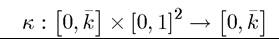
be this best response function, where the the first argument is today’s capital stock and the next two arguments are today’s and tomorrow’s tax rates, so that the function takes the form κ (k, τ, τ⁰), with τ denoting the current tax rate and τ⁰ denoting the tax rate announced for next period.

With this preparation, we can write the maximization problem of a representative en­trepreneur i as follows:

subject to

where I have suppressed expectations, since there will be no uncertainty in this environ­ment (because there are no exogenous shocks and we are focusing on pure strategies). Note thatdenotes the value function of entrepreneur i, when his capital stock

972

(capital-labor ratio) is given by k⅛, those of other entrepreneurs is k, today’s tax rate is τ, and tomorrow’s tax rate has been announced as τ'. In all of this he takes the policy functions of the elite, P, and the best-response function of other entrepreneurs, κ, as given. The con­tinuation value is thereforeHere, k' is his choice

of next period’s capital stock, so it will be the first element of the state variable entering his value function. The capital stock of other entrepreneurs will be given as a function of announced tax rate τ' and according to their best-response function, this isThen

the tax rate announced yesterday becomes the current tax rate, so the third element is and finally, the policy function of the elite implies that they will choose a tax rate for the day after tomorrow as a function of the capital-labor ratio of entrepreneurs then, i.e.,

The entrepreneur’s current level of consumption is then given by (22.37) by standard arguments, with w denoting the equilibrium wage rate. I did not condition on this equilibrium wage rate to reduce the notation which is already quite plentiful.

The maximization by entrepreneur i at each stage simply involves the choice of next date’s capital stock, k'. Let us denote the best response function corresponding to this choice byThe following proposition can be established using the tools from Chapter 6:

Proposition 22.18. Consider the maximization problem in (22.36). For any κ (∙) and P (∙) functions, the value function V is uniquely defined, continuous in all its arguments, and differentiable in the interior of its domain. The optimal policyis defined uniquely

and is continuous in all of its arguments.

Proof. See Exercise 22.16. ?

While the analysis in this section is considerably more complicated than in the models presented so far, Proposition 22.18 is a significant step towards characterizing the equilibrium of this more general economy. In particular, once we have the optimal policy of individual entrepreneur i, k' (k, τ, τ'), it becomes apparent that this optimal policy of individual entre­preneur is the same as the best response function of all entrepreneurs, i.e.,

Therefore we have managed to characterize the behavior of the entrepreneurs in a Markov Perfect Political Economy Equilibrium. Our next step is to take this best response function as given and solve the problem of the elite in setting taxes. For this purpose, let us now write the payoff to the elite recursively. Letbe the value function of the elite when

the current capital-labor ratio chosen by the entrepreneurs is k and the current tax rate is τ. Those are the only two states variables relevant for the elite. In addition, we condition this value function on κ, since this determines how entrepreneurs will react to different tax rates. To simplify the analysis, let us assume that the elite do not have access to any saving 973

technology, thus they have to consume their current tax revenue and also normalize θ^e = 1 without loss of generality. Then their value function can be written as

Intuitively, in the current period, the elite receive a pre-determined amount of tax revenue given by the tax rate, τ, announced in the previous period times output produced by the the capital stock on the economy (which is also predetermined). The capital stock of the economy is equal to the capital-labor ratio of the representative entrepreneur, since the total labor force is equal to 1 (and we have assumed (22.6) so that there is full employment). Next period’s value is then given by the tax rate announced now, τ⁰, and the capital-labor ratio choice of the entrepreneurs given by

The next proposition is again established using the tools from Chapter 6.

Proposition 22.19. The value function given in (22.38) is uniquely defined and is con­tinuous in k and τ.

Proof. See Exercise 22.17. ?

Unfortunately, this proposition does not establish that the value function W is concave or differentiable. This is because it does depend on the function κ (k, τ, τ⁰), which itself may be non-convex. Nevertheless, to make progress with the analysis in the simplest possible way, let us suppose that W is indeed differentiable in both k and τ, and also that κ (k, τ, τ⁰) is differentiable in all three of its arguments. To write the first-order condition for the choice of the tax rate by the elite, let us denote the partial derivatives of the W and κ functions with respect to their jth argument by Wj and Kj, so that, for example, the derivative of W with respect to τ is denoted by W2, etc. Then the first-order condition takes the form

As in Chapter 6, to make further progress, we need to evaluate the two derivatives of the value function in the first-order condition, and we do this by differentiating the value function with respect to k and τ, which gives and

Now taking both expressions to the next period (from t to t +1), and substituting for these, we obtain the following condition for the utility-maximizing tax rate choice of the elite:

974

withThis first-order condition has some similarity to (22.16) from

Section 22.2, but is clearly much more complicated. As with that expression, it trades off the gain from additional taxation,against the loss that additional taxation will

induce by reducing the equilibrium capital-labor ratio (the second term in the first bracket in first line). The second line represents the discounted future change in value arising from the fact that a different tax rate changes the capital-labor ratio tomorrow. Notice that these terms depend both on the best response function of the entrepreneurs, κ, and also on the policy function that the elite will use in the continuation game, P. In general, it is not possible to obtain closed-form solutions for the equilibrium tax rate. The presence of the current capital-labor ratio, k, indicates that the utility-maximizing tax rate will not be a constant. Instead, the equilibrium taxes will evolve over time together with the equilibrium capital-labor ratio.

Unfortunately, a further characterization of equilibrium is not possible without imposing further structure. Typically these types of models are solved under a variety of simplifying assumptions (such as quadratic utility) or the equilibrium is characterized numerically. Even though this more general model does not yield an explicit characterization of the Markov Perfect Political Economy Equilibrium, it highlights the new forces that arise once we in­corporate the transitional dynamics in individual entrepreneurs’ investment decisions, which, in turn, make it optimal for the elite to choose a non-constant path of taxes. However, since there is full depreciation of capital here, some simple cases still enable explicit solutions and Exercise 22.18 discusses a special case with logarithmic preferences and a Cobb-Douglas production function.

22.6.