Heterogeneous Preferences, Social Choice and the Median Voter*
My next objective is to relax the focus on simple societies, which ensured that the social conflict was between the elite and the entrepreneurs. Instead, I wish to illustrate how a richer and more realistic form of heterogeneity among the members of the society will influence policy choices.
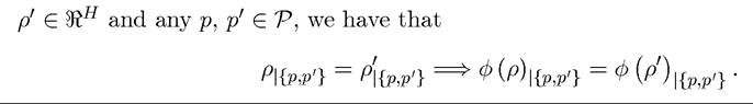
I will do this in two steps. In this section, I will provide a brief overview of how to deal with aggregation of preferences in a society with heterogeneous agents. The celebrated Arrow’s Impossibility Theorem, which we will see shortly, states that this is not possible in general. Nevertheless, under some further assumptions on the structure of preferences (and limits on the menu of available policy options) such aggregation is possible. The main tool in this context, which has wide-ranging applications in political economy models, is the Median Voter Theorem, and its cousin, the Downsian Policy Convergence Theorem. I will show that these two theorems together provide a useful characterization of democratic politics under (limited) heterogeneity among agents. Then, in the next section, using these results I will show that the qualitative results derived in Section 22.2 generalize to a model with 975heterogeneity among entrepreneurs. The bottom line of the analysis in the next section will be that the source of distortionary (“inefficient”) policies that arise from the desire of the political system to extract revenues from a subset of the population is quite a bit more general than in the simple society investigated in Section 22.2. But before doing this, we will get a modicum of basic social choice theory. Strictly speaking, only a simple form of the Median Voter Theorem is necessary for next section, and some of the results here are abstract, hence this section has a “*”.
The Median Voter Theorem (MVT) has a long pedigree in economics and has been applied in many different contexts.
Given its wide use in political economy models, I will start with a section stating and outlining this theorem. I will also take this opportunity to provide a brief statement and proof of Arrow’s Theorem, because this theorem makes the value of the MVT more transparent. I will then emphasize that the MVT, despite its simplicity and elegance, is of limited use, because it only applies to situations in which the menu of policies can be reduced such that the disagreement among all the individuals and society is over a onedimensional (or essentially one-dimensional) policy choice. In situations where the society has to make multiple-dimensional decisions, such as tax on capital and labor or nonlinear income taxation, we cannot use the MVT. I will end this section by outlining some alternative ways of aggregating heterogeneous preferences in such cases, which will also illustrate why in many circumstances the determination of political equilibria can be represented as the maximization of a weighted social welfare function.22.6.1. Basics. This subsection gives an introductory treatment of the large area of social choice theory. Social choice theory is concerned with the fundamental question of political economy already discussed at the beginning of this chapter: how to aggregate the preferences of heterogeneous agents over policies (collective choices). Differently from the most common political economy approaches, however, social choice theory takes an axiomatic approach to this problem. Nevertheless, a quick detour into social chose theory as an introduction to the Median Voter Theorem is useful.
Let us consider an abstract economy consisting of a finite set of individuals denoted by H. We denote the number of individuals by H. Individual i ∈ H has a utility function

Here Xi is his action, with a set of feasible actions denoted by Xi; p denotes the vector of political choices (institutions, policies, other collective choices etc.), with the menu of policies denoted by P; and Y (x,p) is a vector of general equilibrium variables, such as prices or externalities that result from all agents’ actions as well as policy, and X is the vector of the Xi’s.
Instead of writing a different utility function Ui for each agent, I have parameterized the differences in preferences by the variable αg. This is without loss of any generality (simply 976define Ui (∙) ? Ui (∙ | α⅛)) and is convenient for some of the analysis that will follow. Clearly, the general equilibrium variables, such as prices, represented by Y (x,p) here, need not be uniquely defined for a given set of policies p and vector of individual choices x. Since multiple equilibria are not our focus here, we ignore this complication and assume that Y (x,p) is uniquely defined.
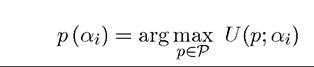
We also assume that, given aggregates and policies, individual ob jective functions are strictly quasi-concave so that each agent has a unique optimal action Xi (p, Y (x,p),α⅛) = argmaxx∈χi u (xi,Y (x,p),p | α⅛). Substituting this maximizing choice of individual i into his utility function, we obtain his indirect utility function defined over policy as U (p; αj). Next define the preferred policy, or the (political) bliss point, of voter i as
In addition, we can think of a more primitive concept of individual preference orderings, which captures the same information as the utility function U (p; αj). In particular, if indi
In this context, we can also think of a “political system” as a way of aggregating the set of utility functions, U (p; αi)'s, to a social welfare function Us (p) that ranks policies for the society. Put differently, a political system is a mapping from individual preference orderings to a social preference ordering. Arrow’s Theorem shows that if this mapping satisfies some relatively weak conditions, then social preferences have to be “dictatorial” in the sense that they will exactly reflect the preferences of one of the agents.
We first present this theorem.22.6.2. Arrow’s (Im) Possibility Theorem. Let us simplify the discussion by assum- 
Let be the set of all reflexive and complete binary relations on P (but notice not necessarily transitive). A social ordering is
 i.e., it is a reflexive complete binary
relation over all the policy choices in P. Thus, a social ordering can be represented as
This mathematical formalism implies that φ (ρ) gives the social ordering for the preference profiles in ρ. We can alternatively think of φ as a political system mapping individual preferences into a social choice. A trivial example of φ is the dictatorial ordering making agent 1 the dictator, so that for any preference profile , φ induces a social order that
entirely coincides with R1.
Note that our formulation already imposes the condition of “unrestricted domain,” which says that in constructing a social ordering we should consider all possible (transitive) individual orderings. Therefore, we are not limiting ourselves to a special class of individual orderings, such as those with “single-peaked” preferences as we will do later in this section.
We say that a social ordering is weakly Paretian i!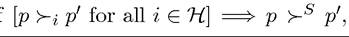
that is, if all individuals in the society prefer p to p', than the social ordering must also rank p ahead of p'. This is weakly Paretian (rather than strongly), since we require all agents to strictly prefer p to p'.
and a singleton, then its unique element is a dictator, meaning that social choices will exactly reflect his preferences regardless of the preferences of the other members of the society. In this case, we say that a social ordering φ is dictatorial.
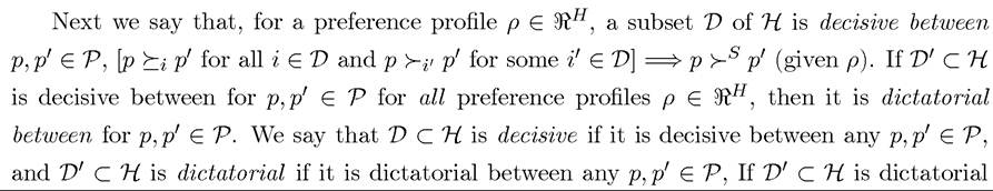
Next a social ordering satisfies independence from irrelevant alternatives if for any ρ and
The axiom of independence from irrelevant alternatives is essential for Arrow’s Theorem. It states that if two preference profiles have the same choice over two policy alternatives, the social orderings that derive from these two preference profiles must also have identical choices over these two policy alternatives, irrespective of how these two preference profiles differ for “irrelevant” alternatives. While this condition (axiom) at first appears plausible, it is in fact a reasonably strong one. In particular, it rules out any kind of interpersonal “cardinal” comparisons—i.e., it excludes information on how strongly an individual prefers one outcome versus another.
The main theorem of the field of social choice theory is the following:
Theorem 22.1. (Arrow's (Im)Possibility Theorem) If a social ordering, φ, is transitive, weakly Paretian and satisfies independence from irrelevant alternatives, then it is dictatorial.
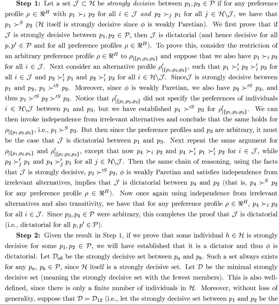
Proof. Suppose to obtain a contradiction that there exists a non-dictatorial and weakly Paretian social ordering, φ, satisfying independence from irrelevant alternatives. We will derive a contradiction in two steps.
979
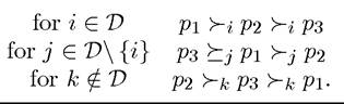
minimal strongly decisive set). If D a singleton, then Step 1 applies and implies that φ is dictatorial, completing the proof. Thus suppose that Then by unrestricted domain, the following preference profile (restricted to {p1,p2jp3}) is feasible
An immediate implication of this theorem is that any set of minimal decisive individuals D within the society H must either be a singleton, that is, D = {i}, so that we have a dictatorial social ordering, or we have to live with intransitivities.
While this theorem is often referred to as Arrow’s Possibility Theorem, it is really an “Impossibility Theorem”. An alternative way of stating the theorem is that there exists no social ordering that is transitive, weakly Paretian, consistent with independence from irrelevant alternatives and non-dictatorial. Viewed in this light, an important implication of this theorem is that there is no way of avoiding the issue of conflict in preferences of individuals by positing a social welfare function. A social welfare function, respecting transitivity, can only replace the actual political economic process of decision making when it is dictatorial. Naturally, who will become the dictator in the society fundamentally brings back the issue of political power, which is also essential for any positive political economy analysis of collective decision-making. In addition, from a modeling point of view, Arrow’s theorem means that, if we are interested in non-dictatorial (and transitive) outcomes, we have to look at political systems that either restrict choices or focus on more concrete situations, where we have to be more specific about the distribution of political power and the vertical institutions regulating the decision-making process. This will be the basis of our analysis for the rest of this chapter and for the next chapter.
Often, economic models restrict the policy space and/or preferences of citizens in order to ensure that this impossibility theorem does not apply. Unfortunately, such restrictions on the policy space have more than technical implications. For example, they often force the modeler to restrict agents to use inefficient methods of redistribution. As a result, some of the inefficiencies that are found in political economy models are not a consequence of the logic of these models, but a consequence of the technical assumptions that the modelers 980
make in restricting the policy space to a single policy. In some circumstances, limits on fiscal instruments might be justified on economic grounds. For example, the assumption that there was only a linear tax on output in Section 22.2 was justified with the argument that lump-sum taxes were not possible. Whether or not this is the case, it is important to recognize that the limits on the set of fiscal instruments is often responsible for the potential distortions resulting from political economy (as was the case in Section 22.2).
One reaction to Arrow’s Theorem might be that the problem of creating individual preferences in this theorem arises because we are not looking at more relevant mechanisms such as voting. The next subsection shows that the same problems arise when collective choices are made by voting. In fact Arrow’s Theorem applies to any possible way of aggregating individual preferences, and if voting were able to solve the problems raised by the theorem, it would be a contradiction to the theorem! Nevertheless, voting can be useful in situations whether we put more structure on preferences and on how individuals vote, which will essentially amount to either giving up the “unrestricted domain” assumption on choices or relaxing the independence from irrelevant alternatives.
22.6.3. Voting and the Condorcet Paradox. Let us illustrate how voting also runs into exactly same problems as those highlighted by Arrow’s Theorem by using a well-known example, the Condorcet paradox. The underlying reason for this paradox is related to Arrow’s Theorem and will also illustrate why, to obtain the Median Voter Theorem below, we will have to introduce reasonably strong restrictions.
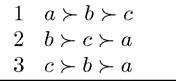
EXAMPLE 22.1. Imagine a society consisting of three individuals, 1, 2, and 3 and three choices. The individuals’ preferences are as follows:
Moreover, let us make the political mechanism somewhat more specific, and assume that it satisfies the following three requirements, which together make up the “open agenda direct democracy” system.
A1. Direct democracy. The citizens themselves make the policy choices via majoritarian voting.
A2. Sincere voting. In every vote, each citizen votes for the alternative that gives him the highest utility according to his policy preferences (indirect function) This
This
requirement is now adopted for simplicity. In many situations, individuals may vote for the outcome that they do not prefer, anticipating the later repercussions of this choice (we refer to this type of behavior as “strategic voting”). Whether they do so or not is important in certain situations, but not for the discussion at the moment.
A3. Open agenda. Citizens vote over pairs of policy alternatives, such that the winning policy in one round is posed against a new alternative in the next round and the set of alternatives includes all feasible policies. Later, we will replace the open agenda assumption with parties offering policy alternatives, thus moving away from direct democracy some way towards indirect/representative democracy. For now it is a good starting point.
Now, using the three assumptions, consider a contest between policies a and b. In this contests, agents 2 and 3 will vote for b over a, so b is the majority winner. Next, by the open agenda assumption, the other policy alternative c will run against b. Now agents 1 and 3 prefer c to b, which is the new majority winner. Next, c will run against a, but now agents 1 and 2 prefer a, so a is the majority winner. Therefore, in this case we have “cycling” over the various alternatives, or put differently there is no “equilibrium” of the voting process that selects a unique policy outcome.
For future reference, let us now define a Condorcet winner as a policy choice that does not lead to such cycling. In particular,
Definition 22.1. A Condorcet winner is a policy p* that beats any other feasible policy in a pairwise vote.
In light of this definition, there is no Condorcet winner in the example of the Condorcet paradox.
22.6.4. Single-Peaked Preferences. Suppose now that the policy space is unidimensional, so that p is a scalar, i.e., P ⊂ R. In this case, a simple way to rule out the Condorcet paradox is to assume that preferences are single peaked for all voters. We will see below that the restriction that P is unidimensional is very important and single-peaked preferences are not well defined when there are multiple policy dimensions.
We say that voter i has single-peaked preferences if his preference ordering for alternative policies is dictated by their relative distance from his bliss point, p(α⅛): a policy closer to p(αi) is preferred over more distant alternatives. Specifically:
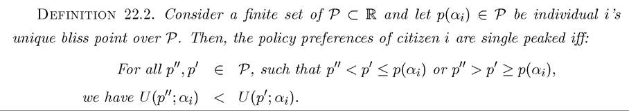
Note that strict concavity of is sufficient for it to be single peaked, but is not necessary. In fact, single-peakedness is equivalent to strict quasi-concavity. This definition could be weakened so that the bliss point of the individual is not unique (i.e., from strict quasiconcavity to quasi-concavity). But this added generality is not important for our purposes.
982
We can easily verify that in the Condorcet paradox, not all agents possessed single-peaked preferences. For example, taking the ordering to be a, b, c, agent 1 who has preferences 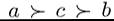 does not have single-peaked preferences (if we took a different ordering of the alternatives, then the preferences of one of the other two agents would violate the single- peakedness assumption, see Exercise 22.21).
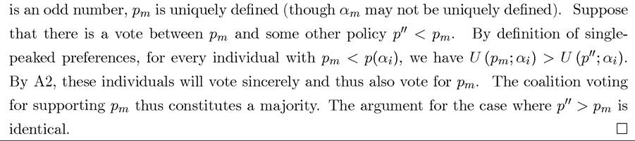
The next theorem shows that with single-peaked preferences there always exists a Condorcet winner. Before stating this theorem, let us define the median voter of the society. Given the assumption that each individual has a unique bliss point over P, we can rank all individuals according to their bliss points, the Also, to remove uninteresting ambiguities, let us imagine that H is an odd number (i.e., H consists of an odd number of individuals). Then the median voter is the individual who has exactly (H — 1) /2 bliss points to his left and (H — 1) /2 bliss points to his right. Put differently, his bliss point is exactly in the middle of the distribution of bliss points. We denote this individual by αm, and his bliss point (ideal policy) is denoted by pm.
Theorem 22.2. (The Median Voter Theorem) Suppose that H is an odd number, that A1 and A2 hold, and that all voters have single-peaked policy preferences over a given ordering of policy alternatives, P. Then, a Condorcet winner always exists and coincides with the median-ranked bliss point, pm. Moreover, pm is the unique equilibrium policy (stable point) under the open agenda majoritarian rule, that is, under A1-A3.
Proof. The proof is by a “separation argument”. Order the individuals according to their bliss points p(αi), and label the median-ranked bliss point by pm. By the assumption that H
The assumption that the society consists of an odd number of individuals was made only to shorten the statement of the theorem and the proof. Exercise 22.23 asks you to generalize the theorem and its proof to the case in which H is an even number.
More important than whether there are an odd or even number of individuals in the society is the assumption of sincere voting. Clearly, rational agents could deviate from truthful reporting of their preferences (and thus from truthful voting) when this is beneficial for them. So an obvious question is whether the MVT generalizes to the case in which individuals do not vote sincerely? The answer is yes. To see this, let us modify the sincere voting assumption to strategic voting:
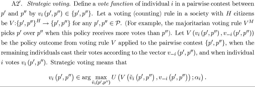
In other words, strategic voting implies that each individual chooses the voting strategy that maximizes utility given the voting strategies of other agents.
Finally, recall that a weakly-dominant strategy for individual i is a strategy that gives weakly higher payoff to individual i than any of his other strategies irrespective of the strategy profile played by all other players
Theorem 22.3. (The Median Voter Theorem With Strategic Voting) Suppose that H is an odd number, that A1 and A20 hold, and that all voters have single-peaked policy preferences over a given ordering of policy alternatives, P. Then, there exists a weakly- dominant strategy for each player to vote sincerely and in this equilibrium, the median-ranked bliss point, pm is the Condorcet winner.
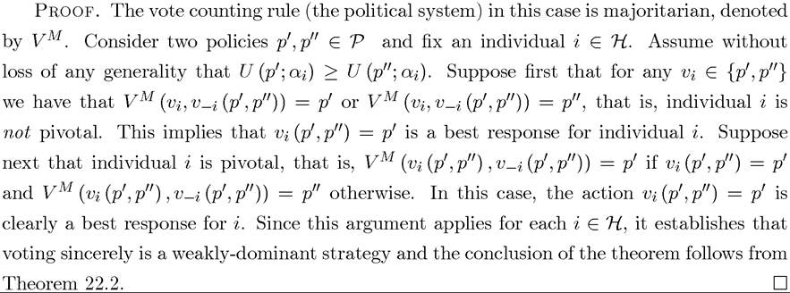
Notice that the second part of the Theorem 22.2, which applied to open agenda elections, is absent in Theorem 22.3. This is because the open agenda assumption does not lead to a well defined game, so a game theoretic analysis and thus an analysis of strategic voting is no longer possible.
In fact, there is no guarantee that sincere voting is optimal in dynamic situations even with single-peaked preferences. The following example illustrates this:
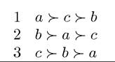
EXAMPLE 22.2. Consider three individuals with the following preference orderings.
These preferences are clearly single peaked (order them alphabetically to see this). In a one round vote, b will beat any other policy. But now consider the following dynamic voting set up: first, there is a vote between a and b. Then, the winner goes against c, and the winner of this contest is the social choice. Sincere voting will imply that in the first round players 2 and 3 will vote for b, and in the second round, players 1 and 2 will vote for b, which will become the social choice.
Is such sincere voting “equilibrium behavior” ? Exactly the same argument as above shows that in the second round, sincere voting is a weakly dominant strategy. But not necessarily in round one. Suppose players 1 and 2 are playing sincerely. Now if player 3 deviates and votes for a (even though she prefers b), then a will advance to the second round and would lose to c. Consequently, the social choice will coincide with the bliss point of player 3. Exercise 22.24 asks you to characterize the subgame perfect equilibrium of this game under strategic voting by all players.
Dynamic voting issues become more interesting, and open the way for agenda setting, when there are no Condorcet winners. The following example illustrates this.
EXAMPLE 22.3. Consider the preference profile in Example 22.1 and the following political mechanism. First, all individuals vote between a and b, and then they vote over the winner of this contest and c. With sincere voting, b will win the first round, and then c wins the second round against b. Now consider agent 2. If he changes his vote in the first round to a (thus does not vote sincerely), the first-round winner will be a, which will also win against c, and player 2 prefers this outcome to the outcome of sincere voting, which was c.
This example can also be used to illustrate the role of “agenda setting”. Suppose that in the above game, agent 1 decides the exact orderings of voting. In particular, he has to choose between three options (a vs. b first, a vs. c first, and b vs. c, first). Anticipating strategic voting by player 2, he will choose the first option and will ensure that his most preferred alternative becomes the political choice of the society. In contrast, if agent 3 chose the ordering, he would go for a vs. c first, which would induce agent 1 to vote strategically for c, and lead to c as the ultimate outcome.
22.6.5. Party Competition and the Downsian Policy Convergence Theorem. The focus so far has been on voting between two alternative policies or on open agenda voting, which can be viewed as an extreme form of “direct democracy”. The MVT becomes potentially more relevant and more powerful when applied in the context of indirect democracy, that is, when combined with a simple model of party competition. We now give a brief 985
overview of this situation and derive the Downsian Policy Convergence Theorem, which is the basis of much applied work in political economy.
Suppose that we have a situation in which there is a Condorcet winner, and there are two parties, A and B, competing for political office. Assume that the parties do not have an ideological bias, and would like to come to power (for example, they receive some utility from being in power). In particular, they both maximize the probability of coming to power, for example, because they receive a rent or utility of Q > 0 when they are in power.
Assume also that parties simultaneously announce their policy, and are committed to this policy. This implies that the behavior of the two parties can be represented by the following pair of maximization problems:
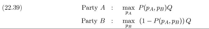
where Q denotes the rents of being in power and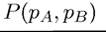 is the probability that party
A comes to power when the two parties’ platforms are pr↑ and p>∣> respectively. When the median voter theorem applies, and denoting the bliss point of the median voter by pm, we have
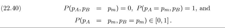
This last statement follows since when both parties offer exactly the same policy, it is the best response for all citizens to vote for either party. However, the literature typically makes the following assumption:
A4. Randomization:
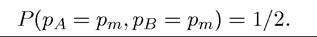
This assumption can be rationalized by arguing that when indifferent individuals, randomize between the two parties, and since there are many many individuals, by the law of large numbers, each party obtains exactly half of the vote.
We then have the following result:
Theorem 22.4. (Downsian Policy Convergence Theorem) Suppose that there are two parties that first announce a policy platform and commit to it and a set of voters H that vote for one of the two parties. Assume that Af holds and that all voters have single-peaked policy preferences over a given ordering of policy alternatives, and denote the median-ranked bliss point by pm. Then both parties will choose pm as their policy platform.
Proof. The proof is by contradiction. Suppose not, then there is a profitable deviation for one of the parties. For example, one of the parties can announce pm
986
and win the election for sure. party A can also announce pm
and increase its chance of winning to 1/2. ?
Exercise 22.25 asks you to provide a generalization of this theorem without Assumption A4.
This theorem is important because it demonstrates that there will be policy convergence between the two parties and that party competition will implement the Condorcet winner among the voters. Therefore, in situations in which the MVT applies, the democratic process of decision making with competition between two parties will lead to a situation in which both parties will choose their policy platform to coincide with the bliss point of the median voter. Thus the MVT and the Downsian Policy Convergence Theorem together enable us to simplify the process of aggregating the heterogeneous preferences of individuals over policies and assert that, under the appropriate assumptions, democratic decision-making will lead to the most preferred policy of the median voter. The Downsian Policy Convergence Theorem is useful in this context, since it gives a better approximation to “democratic policymaking” in practice than open agenda elections.
There is a sense in which Theorem 22.4 is slightly misleading, however. While the theorem is correct for a society with two parties, it gives the impression of a general tendency towards policy convergence in all democratic societies. Many democratic societies have more than two parties. A natural generalization of this theorem would be to consider three or more parties. Unfortunately, as Exercise 22.26 shows the results of this theorem do not generalize to three parties. Thus some care is necessary in applying the Downsian Policy Convergence Theorem without regards to existing political institutions of the society.
Another obvious question is what would happen in the party competition game when there is no Condorcet winner. Theorem 22.4 does not generalize to this case either. In particular, if we take a situation in which there is “cycling,” like the above Condorcet paradox example, it is straightforward to verify that there is no pure strategy equilibrium in the political competition game. This is further discussed in Exercise 22.27.
22.6.6. Beyond Single-Peaked Preferences. Single-peaked preferences played a very important role in the results of Theorem 22.2 by ensuring the existence of a Condorcet winner. However, single peakedness is a very strong assumption and does not have a natural analog in situations in which voting is over more than one policy choice. When there are multiple policy choices (or even voting over “functions” such as nonlinear taxation), much more structure needs to be imposed over voting procedures and agenda setting to determine equilibrium policies. Those issues are beyond the scope of our treatment here. Nevertheless, it is possible to relax the assumption of single-peaked preferences, and also introduce a set of preferences that are “close” to single-peaked in multidimensional spaces. The latter task would take us 987
too far afield from our focus, so will be left to Exercise 22.28. Here we introduce the useful concept of single-crossing property, which will enable us to prove a version of Theorem 22.2 under somewhat weaker assumptions.
Definition 22.3. Consider an ordered policy space P and also order voters according to their ai's. Then the preferences of voters satisfy the single-crossing property over the policy space P when the following statement is true:
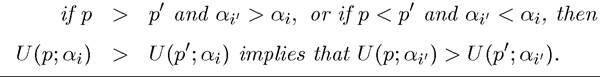
EXAMPLE 22.4. To see why single-crossing property is weaker than single-peaked preferences, consider the following example: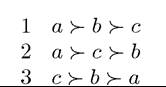
It can be verified easily that these preferences are not single peaked. The natural ordering is a > b > c, but in this case the preferences of player 2 have two peaks, at a and c. To see why these preferences satisfy single crossing, take the same ordering, and also order players as 1, 2, 3. Now we have
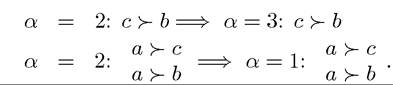
Notice that while single peakedness is a property of preferences only, the single-crossing property refers to a set of preferences over a given policy space P. It is therefore a joint property of preferences and choices. The following theorem generalizes Theorem 22.2 to a situation with single crossing.
Theorem 22.5. (Extended Median Voter Theorem) Suppose that A1 and A2 hold and that the preferences of voters satisfy the single-crossing property. Then a Condorcet winner always exists and coincides with the bliss point of the voter with the median value am.
Proof. The proof works with exactly the same separation argument as in the proof of Theorem 22.2. Consider the median voter with αm, and bliss policy pm. Consider an
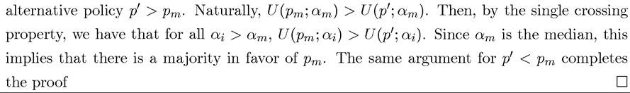
Given this theorem, the following result is immediate:
Theorem 22.6. (Extended Downsian Policy Convergence) Suppose that there are two parties that first announce a policy platform and commit to it and a set of voters that vote for one of the two parties. Assume that Af holds and that all voters have preferences that satisfy the single-crossing property, and denote the median-ranked bliss point by pm. Then both parties will choose pm as their policy.
Proof. See Exercise 22.27. ?
Despite this generalization, which is quite useful in many applications, and the extension of the MVT presented in Exercise 22.28, the MVT-type results do not apply in many situations with multi-dimensional policies. Exercise 22.29 gives a simple example, which illustrates how widespread the failure of the MVT will be in practice.
22.6.7. Equilibrium Social Welfare Functions. The MVT and the Downsian Policy Convergence Theorems are powerful for the analysis of many models of political economy. However, as Exercise 22.29 illustrates, the assumptions necessary for these theorems do not apply in many interesting (even simple) models. The political economy literature has thus considered a variety of other plausible ways of aggregating heterogeneous preferences within democratic contexts. Three particularly popular approaches are (1) the “probabilistic voting” models, which essentially add some noise in the voting behavior of individuals (for example, because individuals care about some other non-policy characteristic of the parties that are competing for office); (2) models without policy commitment, such as the citizen-candidate models, in which voters elect a politician, who then decides the policies after election; (3) lobbying models, in which some of the individuals or groups in the society can spend money in order to influence the outcome of democratic politics. A full analysis of these models is beyond the scope of the current book. Nevertheless, one feature of many of these formulations is worth noting, especially in light of the discussion of the issue of Pareto efficiency above. Many simple versions of these models lead to equilibria that are equivalent to maximizing a “reduced-form weighted social welfare function”. The form of this social welfare function is derived from the political economy equilibrium and depends on the specific assumptions made in these models. For our purposes, the noteworthy point is that in some situations, the political economy equilibrium involves maximizing a weighted social welfare function (given the set of policy instruments), as we have done in Sections 22.2-22.4. We now discuss two standard models that leads to this type of equilibrium (weighted) social welfare functions.
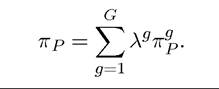
22.6.7.1. Probabilistic Voting and Swing Voters. Let the society consist of G distinct groups of voters, with all voters within a group having the same economic characteristics and preferences. As in the Downsian model, there is electoral competition between two parties, A and B, and let be the fraction of voters in group g voting for party P where P = A, B, and let λg be the share of voters in group g and naturally
 Then the expected vote share of party P is
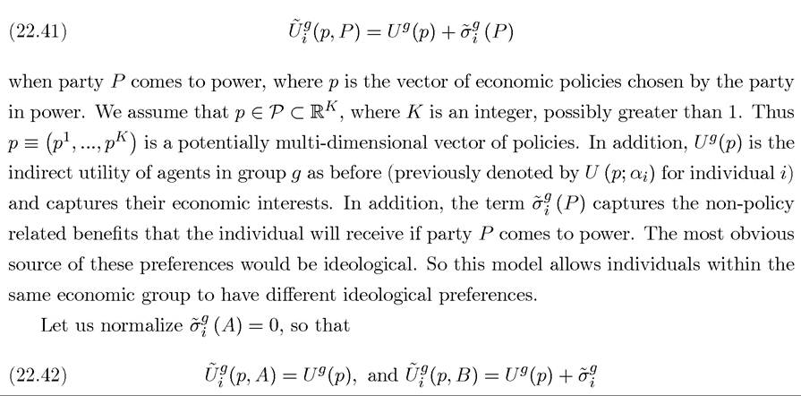
In our analysis so far, all voters in group g would have cast their votes identically (unless they were indifferent between the two parties). The idea of probabilistic voting is to smooth out this behavior by introducing other considerations in the voting behavior of individuals. Put differently, probabilistic voting models will add “noise” to equilibrium votes, smoothing the behavior relative to models we analyzed so far. In particular, suppose that individual i in group g has the following preferences:
In that case, the voting behavior of individual i can be represented as 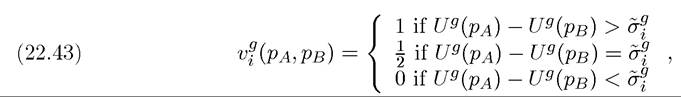 where
where denotes the probability that the individual will vote for party A, pa is the
platform of party A and đâ is the platform of party B, and as above, we have assumed that if an individual is indifferent between the two parties (inclusive of the ideological benefits), he randomizes his vote.
Let us now assume that the distribution of non-policy related benefits for individual i in group g is given by a smooth cumulative distribution function Hg defined over (-∞, +∞), with the associated probability density function hg. The draws of
 across individuals are independent. Consequently, the vote share of party A among members of group g is
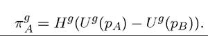
Furthermore, to simplify the exposition here, suppose that parties maximize their expected vote share. In this case, party A sets this policy platform pa to maximize:
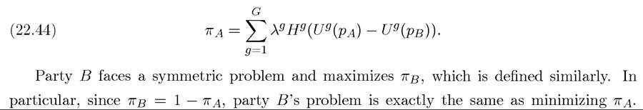
Equilibrium policies will then be determined as the Nash equilibrium of a (zero-sum) game where both parties make simultaneous policy announcements to maximize their vote share. Let us first look at the first-order condition of party A with respect to its own policy choice, PA, taking the policy choices of the other party, đâ, as given. This is:
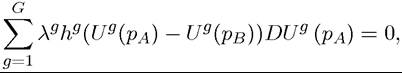
where DUg (pa) is the gradient of Ug (∙) given by
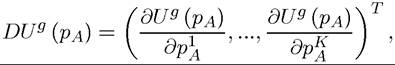
with pA corresponding to the kth component of the policy vector pa. Since the problem of party B is symmetric, it is natural to focus on pure strategy symmetric equilibria. In fact, if the maximization problems of both parties are strictly concave, such a symmetric equilibrium will exist (see Exercise 22.30). Clearly in this case, we will have policy convergence with PA = PB = P*, and thus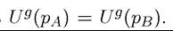 Consequently, symmetric equilibrium policies,
announced by both parties, must be given by
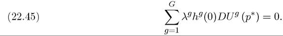
It is now straightforward to see that equation (22.45) also corresponds to the solution to the maximization of the following weighted utilitarian social welfare function:
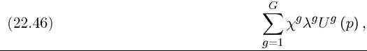

Theorem 22.7. (Probabilistic Voting Theorem) Consider a set of policy choices P, 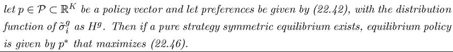
The important point to note about this result is its seeming generality: as long as a pure strategy symmetric equilibrium in the party competition game exists, it will correspond to a maximum of some weighted social welfare function. This generality is somewhat exaggerated, however, since such a symmetric equilibrium does not always exists. In fact, conditions to guarantee existence of pure strategy symmetric equilibria are rather restrictive and are discussed in Exercise 22.30.
22.6.7.2. Lobbying. Consider next a very different model of policy determination, a lobbying model. In a lobbying model, different groups make campaign contributions or pay money to politicians in order to induce them to adopt a policy that they prefer. With lobbying, political power comes not only from voting, but also from a variety of other sources, including whether various groups are organized, how much resources they have available, and their marginal willingness to pay for changes in different policies. Nevertheless, the most important result for us will be that even with lobbying, equilibrium policies will look like the solution to a weighted utilitarian social welfare maximization problem.
To see this, we will quickly review the lobbying model due to Grossman and Helpman (1996). Imagine again that there are G groups of agents, with the same economic preferences. The utility of an agent in group g, when the policy that is implemented is given by the vector 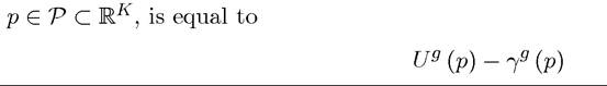 where
where is the usual indirect utility function, and γg (p) is the per-person lobbying contribution from group g. We will allow these contributions to be a function of the policy implemented by the politician, and to emphasize this, it is written with p as an explicit argument.
Following Grossman and Helpman, let us assume that there is a politician in power, and he has a utility function of the form
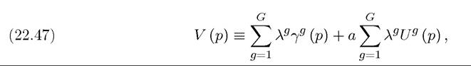
where as before λg is the share of group g in the population. The first term in (22.47) is the monetary receipts of the politician, and the second term is utilitarian aggregate welfare. Therefore, the parameter a determines how much the politician cares about aggregate welfare. When a = 0,he only cares about money, and when a → ∞, he acts as a utilitarian social planner. One reason why politicians might care about aggregate welfare is because of electoral politics (for example, they may receive rents or utility from being in power as in the last subsection and their vote share might depend on the welfare of each group).
Now consider the problem of an individual j in group g. By contributing some money, he might be able to sway the politician to adopt a policy more favorable to his group. But 992
he is one of many members in his group, and there is a natural free-rider problem. He might let others make the contribution, and simply enjoy the benefits. This will typically be an outcome if groups are unorganized (for example, there is no effective organization coordinating their lobbying activity and excluding non-contributing members from some of the benefits etc.). On the other hand, organized groups might be able to collect contributions from their members in order to maximize group welfare.
We will think that out of the G groups of agents, of those are organized as lobbies, and can collect money among their members in order to further the interests of the group. The remaining
 are unorganized, and will make no contributions. Without loss of any generality, let us rank the groups such that groups
 to be the organized ones.
The lobbying game takes the following form: every organized lobby g simultaneously offers a schedule which denotes the payments they would make to the politician
when policy p ∈ P is adopted. After observing the schedules, the politician chooses p. Notice the important assumption here that contributions to politicians (campaign contributions or bribes) can be conditioned on the actual policy that’s implemented by the politicians. This assumption may be a good approximation to reality in some situations, but in others, lobbies might simply have to make up-front contributions and hope that these help the parties that are expected to implement policies favorable to them get elected.
This is a potentially very complex game, since various different agents (here lobbies) are choosing functions (rather than scalars or factors). Nevertheless, the equilibrium of this lobbying game takes a relatively simple form.
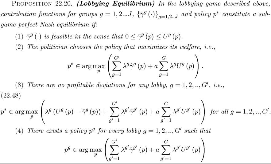
and satisfies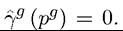 That is, the contribution function of each lobby is such
that there exists a policy that makes no contributions to the politician, and gives her the same utility.
Proof. (Sketch) Conditions 1, 2 and 3 are easy to understand. No group would ever offer a contribution schedule that does not satisfy Condition 1. Condition 2 has to hold, since the politician chooses the policy. If Condition 3 did not hold, then the lobby could change its contribution schedule slightly and improve its welfare. In particular suppose that this condition does not hold for lobby g = 1, and instead of p*, some p maximizes (22.48). Denote the difference in the values of (22.48) evaluated at these two vectors by ∆ > 0. Consider the following contribution schedule for lobby g = 1:

where c1 (p) is an arbitrary function that reaches its maximum at p = p. Following this contribution offer by lobby 1, the politician would choose p = p for any ε > 0. To see this note that by part (1), the politician would choose policy p that maximizes

Since for any ε > 0 this expression is maximized by p, the politician would choose p. The change in the welfare of lobby 1 as a result of changing its strategy is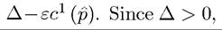 for small enough ε, the lobby gains from this change, showing that the original allocation could not have been an equilibrium.
Finally, condition 4 ensures that the lobby is not making a payment to the politician above the minimum that is required. If this condition were not true, the lobby could reduce its contribution function by a constant, still induce the same behavior, and obtain a higher payoff. ?
Next suppose that these contribution functions are differentiable.4 Then it has to be the case that for every policy choice, pk, within the vector p*, we must have from the first-order condition of the politician that
[1]But there is nothing in the analysis that implies that these functions have to be differentiable; in fact, equilibria with non-differentiable functions are easy to construct. Nevertheless, it is generally thought that equilibria with non-differentiable functions are more “fragile” and thus less relevant. See the discussion in Grossman and Helpman (1994) and Bernheim and Whinston (1986).
and from the first-order condition of each lobby that

Combining these two first-order conditions, we obtain
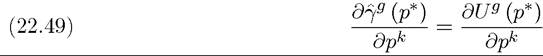
for all k = 1, 2,..,K and g = 1, 2,..,G0. Intuitively, at the margin each lobby is willing to pay for a change in policy exactly as much as this policy will bring them in terms of marginal return.
But then this implies that the equilibrium can be characterized as a solution to maximizing the following function 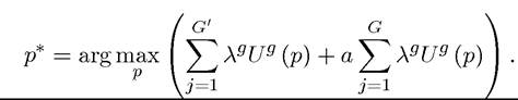
Consequently, the lobbying equilibrium can also be represented as a solution to the maximization of a weighted social welfare function, with individuals in unorganized groups getting a weight of a and those in organized group receiving a weight of 1 + a. Intuitively, 1/a measures how much money matters in politics, and the more money matters, the more weight groups that can lobby receive. As a → ∞, we converge to the utilitarian social welfare function.
22.7.