DistributionalConflict and Economic Growth: Heterogeneity and the Median Voter
Let us now return to the model of Section 22.2 with linear preferences, but relax the assumption that political power is in the hands of an elite. Instead, we will now introduce heterogeneity among the agents and then apply the tools from the previous section, in particular, the Median Voter Theorem, Theorems 22.2 and 22.5, to analyze the political economy of this model.
Recall that these theorems show that if there is a one-dimensional policy choice and individuals have single-peaked preferences (or preferences over the menu of policies that satisfy the single-crossing property), then the political equilibrium will coincide with the most preferred policy of the median voter.To focus on the main issues in the simplest possible way, I will modify the environment from Section 22.2 slightly. First, there are no longer any elites. Instead, economic decisions will be made by democratic voting among all the agents. Second, to abstract from political conflict between entrepreneurs and workers, I will also assume that there are no workers (recall Exercise 22.3 for why having only entrepreneurs simplifies the analysis; see Exercise 22.31 for an economy where individuals differ both in terms of their productivity and occupation).
995
Instead, the economy consists of a continuum 1 of yeoman-entrepreneurs, each denoted by i ∈ [0,1] and with access to a neoclassical production function
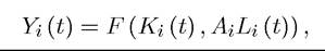
where Ai is a time-invariant labor-augmenting productivity measure and will be the only source of heterogeneity among the entrepreneurs. In particular, F satisfies Assumptions 1 and 2. We assume that Ai has a distribution given by μ (A) among the entrepreneurs. The yeoman-entrepreneur assumption means that each entrepreneur can only employ himself as the worker, so Li (t) = 1 for all i ∈ [0,1] and for all t.
This assumption is important, since otherwise the most productive entrepreneur would hire the entire labor force. Since heterogeneity is the main focus, some way of introducing diminishing returns for each entrepreneur is important, and the yeoman-entrepreneur assumption achieves this in a simple way. I also set the depreciation rate of capital δ equal to 1 to simplify notation.As noted previously, all agents have linear preferences given by (22.1). Linear preferences again simplify the analysis, by separating the political decisions at different periods. As in Section 22.2, the investment decisions at time t + 1 will depend only on the tax rate announced for time t + 1. This latter feature is particularly important here, since we know from the previous section that the Median Voter Theorem does not generally apply with multi-dimensional policy choices. The fact that at each point in time there is only one relevant tax policy will enable us to use the Median Voter Theorem.
More specifically, the timing of events is very similar to that in Section 22.2. At each date t:
We will focus on the Markov Perfect Political Economy Equilibrium of this game.
The important assumption here is that at each stage voting is over the tax rate that will apply in the next period only (with the lump-sum transfer determined from the budget constraint). Moreover, given the linear preferences, each individual takes future taxes as given (independent of current tax decisions and the current capital stock) and only cares about the current tax rate when making its current decisions. Thus, despite the fact that the economy involves an infinite sequence of taxes, the MVT can be applied to the tax decision at each date, provided the other conditions of the theorem are satisfied. We next show that this is the case.
Let us next determine the political bliss point of each entrepreneur, i.e., their most preferred tax rate.
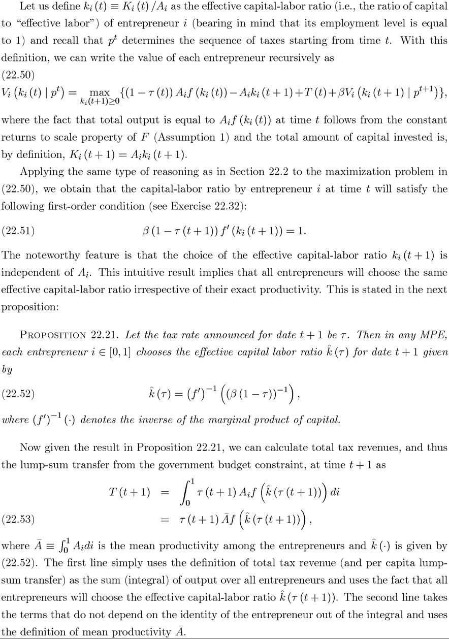
To do this, let us write their continuation utility from the end of period t. Ignoring all the terms that are bygone by this point and substituting for best responses (i.e., for the effective capital-labor ratio from (22.52)), the expected discounted utility of entrepreneur i from (22.50) can be written as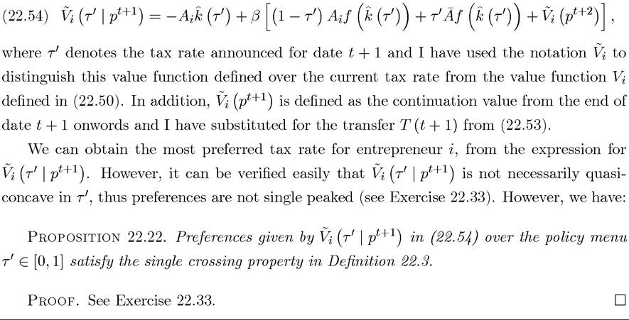
In view of Proposition 22.22, we can apply Theorems 22.5 and 22.6, and conclude that at each date, the tax rate most preferred by the entrepreneur with the median productivity will be implemented. Let this median productivity be denoted by Am. From (22.54), this most preferred tax rate satisfies the following first-order condition:
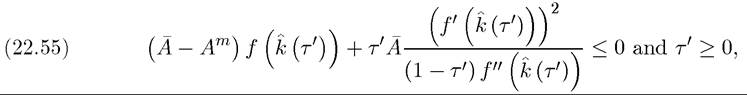
with complementary slackness. In writing this expression, we have made use of condition (22.52) to simplify the expression and also to express the derivative of as
as
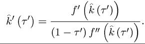
This derivative is strictly negative since f'' < 0. Therefore, as in Section 22.2, higher taxes lead to lower capital-labor ratios and lower output (higher distortions). The emphasis on complementary slackness in (22.55) is important here, since the most preferred tax rate of the median voter (entrepreneur) may not satisfy the first-order condition as equality, instead corresponding to a corner solution of τ' — 0. The next proposition shows that this is in fact relevant for a range of distributions of productivity among the entrepreneurs.
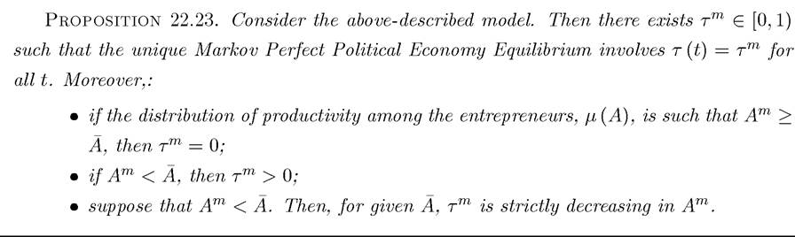
Proof. The argument preceding the proposition combined with Theorems 22.5 and 22.6 shows that the tax rate most preferred by the entrepreneur with the median productivity will be chosen at every period. Moreover, clearly τ' = 1 cannot be preferred by any entrepreneur, since it would lead to zero output by each entrepreneur and thus to zero tax revenues (Exercise 22.1), thus the result that there exists τm ∈ [0,1) such that τ (t) = τm for all t follows, with τm a solution to (22.55).
Note that this equation might have more than one solution, and if so, τm corresponds to the global maximizer of (22.54) with productivity evaluated at Am.Next suppose that Am = A, then the first expression in (22.55) is equal to zero, and the left-hand side of the equation is unambiguously negative for any τ0 > 0 and exactly equal to zero for τ0 = 0. This establishes that in this case τm = 0. If, on the other hand, Am > A, then the first expression is strictly negative and the left-hand side of (22.55) is unambiguously negative and the conclusion that τm = 0 follows from the complementary slackness conditions.
Finally, suppose that Am < A. In this case, the first expression strictly positive. Suppose, to obtain a contradiction, that τm = 0. Then the second term is exactly equal to 0 (since τ0 is in the numerator). Consequently, the left-hand side of (22.55) is strictly positive and τm = 0 cannot be a solution. Hence the unique equilibrium tax rate must be τm > 0. To obtain the comparative static result, simply apply the Implicit Function Theorem to (22.55) and use the fact that since τm is a global maximum, the derivative of (22.55) with respect to τm is negative. ?
There are a number of important results in this proposition. First, it shows that linear preferences guarantee the existence of a well-defined Markov Perfect Political Economy Equilibrium even when there is heterogeneity among the individuals in terms of their productivity. The important role played by linear preferences in this result cannot be overstated (recall Section 22.5). As discussed at the end of this chapter, there are a number of results in the literature similar to this proposition, but they do not correspond to well-defined Markov Perfect Equilibria because they do not feature linear preferences (instead, they can be thought of as the equilibria in which individuals vote once at the beginning of time and have no option to change taxes thereafter).
Second, this proposition shows that if the productivity of the median voter is above the average, there will be no redistributive taxation. This is intuitive. As the first term in (22.55) makes it clear, the benefits of taxation are proportional to the average productivity in the economy, while the cost (to the median voter) is related to his productivity. If the median entrepreneur is more productive than the average, there are two forces making him oppose redistributive taxation; he is effectively redistributing away from himself, and there is also the distortionary effect of taxation captured by the second term in (22.55).
Third and more important, in the case in which the productivity of the median voter is below the average, the political equilibrium will involve positive (distortionary) taxation on all entrepreneurs. To obtain the intuition for this result, recall that taxes revenues are equal to zero at τ = 0. A small increase in taxes starting at τ = 0 has a second-order loss for each entrepreneur and when Am < A, a first-order redistributive gain for the median voter. This result is important in part because most real-world wealth and income distributions appear to be skewed to the left (with the median lower than the mean), thus this configuration is more likely in practice. Furthermore, this result is most interesting in comparison with those in Section 22.2, which also involved positive distortionary taxation, but in an environment in which a non-productive elite was in power. Proposition 22.23 shows that the same qualitative result generalizes to the case in which there is democratic politics and the decisive (median) voter is a productive entrepreneur himself, but is less productive than average. This implies that the essence of the results obtained in our analysis of elite-dominated politics applies much more generally.
Finally, Proposition 22.23 gives a new comparative static result. It shows that, holding average productivity constant, a decline in the productivity of the median entrepreneur (voter) leads to an increase in the amount of distortionary taxes.
Since as in Section 22.2, higher taxes correspond to lower output and the larger gap between the mean and the median of the productivity distribution can be viewed as a measure of inequality, this result suggests a political mechanism via which greater inequality may translate into higher distortions and lower output.Nevertheless, some care is necessary in interpreting this last result, since the gap between the mean and the median is not a (formally appropriate) measure of inequality. Exercise 22.34 gives an example in which a mean preserving spread of the distribution lead to a smaller gap between the mean and the median. This caveat notwithstanding, the literature interprets this last result as suggesting that greater inequality should lead to lower output and lower growth. Exercise 22.35 presents a version of the model here where taxes affect the equilibrium growth rate.
22.8.