Private Consumption and Money Demand in a Representative Household Model

Assume, as in the Ramsey model of chapter 4, a competitive economy in which all households are identical. Households are indexed by j, where j is uniformly distributed between zero and 1.

The number of members of each household is equal to L(t) and is growing at an exogenous rate n, which is also the growth rate of population L(t). Labor supply and employment is equal to L(t), and the efficiency of labor h(t) grows at an exogenous rate of technical progress g. The instantaneous utility function of households depends on consumption of goods and services, and on holdings of real money balances.

7.1.1 Money in the Utility Function of Households

Household j selects a path of consumption and real money balances to maximize the following intertemporal utility function:

The maximization takes place under the instantaneous budget constraint

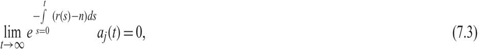
and the transversality condition

where ρ is the pure rate of time preference of households, and u is a quasi-concave instantaneous utility function that depends on consumption and real money balances (assumed positive). In addition, c_j(t) denotes average consumption per person of household j at time t, m_j(t) denotes average per person real money balances of household j at time t, a_j(t) is average assets per person (nonhuman wealth) of household j at time t, w(t) denotes the real wage per efficiency unit of labor at time t, h(t) is labor efficiency per worker, τ(t) denotes average taxes (minus transfers) per efficiency unit of labor at time t, r(t) is the real interest rate at time t, n is the population growth rate (equal to the growth rate of members per household), and π(t) is inflation (which is equal to expected inflation).

Real money balances provide utility because of their liquidity services: they facilitate payments (the exchange of goods and services) and reduce transaction costs. The instantaneous utility function is assumed to take the form

where 1/θ is the intertemporal elasticity of substitution of consumption and real money balances, and γ is the share of consumption in the utility of the household. This utility function, which is a generalization of the constant elasticity of intertemporal substitution (CEIS) utility function we used previously, is additively separable: The elasticity of substitution between consumption and real money balances is equal to unity.

7.1.2 Nominal and Real Interest Rates and the Opportunity Cost of Real Money Balances

Unlike other assets held by households (such as capital or government bonds), the nominal yield of money is equal to zero, because money balances do not pay interest. Moreover, when there is a positive inflation rate π(t), real (inflation adjusted) money balances depreciate at the inflation rate π(t).

Therefore, the opportunity cost of holding real money balances is equal to the sum of the real return of interest-yielding assets plus the expected inflation rate. This is defined as the nominal interest rate i(t), which is determined by

This relationship between nominal and real interest rates is the Fisher equation introduced and discussed in chapter 2. It was first highlighted by Irving Fisher in 1896.³

7.1.3 First-Order Conditions for an Optimum

Maximizing (7.1) under the constraint (7.2) by forming the relevant Hamilton function yields the following first-order conditions:

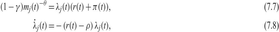
where λ_j(t) is the current value multiplier of the relevant current value Hamilton function, and its economic interpretation is that it measures the shadow value of marginal savings (assets) of the household.

From (7.6), λ_j(t), which is the shadow value of marginal savings, is equal to the current marginal utility of consumption. At the optimum, the marginal value of savings must be equal to the marginal utility of consumption, and the household must be indifferent between consumption and savings.

From (7.7), the current marginal utility of real money balances is equal to the marginal utility of consumption λ_j(t) times the opportunity cost of holding real money balances. At the optimum, the marginal value of holding real money balances must be equal to the opportunity cost of holding money, evaluated in terms of the marginal utility of consumption. Thus, at the optimum, the household should be indifferent between substituting consumption for the utility services of money.

Finally, from (7.8), the marginal utility of consumption falls at a rate equal to the difference between the real interest rate and the pure rate of time preference. This is another way of saying that the expected real return on savings, including capital gains on assets, is equal to the pure rate of time preference of the household. This can be seen by rearranging (7.8):

As shown below, we can now use the first-order conditions to derive the money demand function and the Euler equation for consumption.

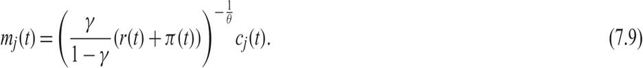
7.1.4 The Money Demand Function

Dividing (7.7) by (7.6) and solving for real money balances, we can derive a function for the demand for real money balances by the representative household:

We can use (7.9) to deduce aggregate money demand. Multiplying both sides of (7.9) by L(t), we get

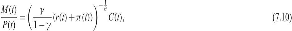
where M(t) is the aggregate nominal money supply, P(t) is the price level, and C(t) is aggregate real consumption of goods and services.

Equation (7.10) is characterized by homogeneity of degree one with respect to the price level, because households demand money for its purchasing power. For a given aggregate real consumption and nominal interest rates, doubling the money supply would cause a doubling of the price level. This property is known as the neutrality of money.

Expressing real money balances per efficiency unit of labor, we have

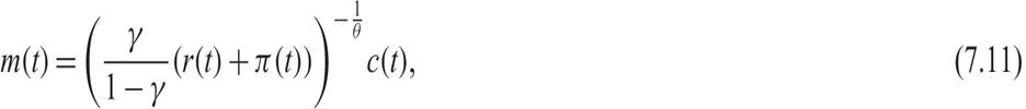
where c = C/hL, m = (M/P)/hL, and h is the efficiency of labor.

7.1.5 Growth Rate of the Money Supply and Inflation

One can use (7.10) or (7.11) to determine the price level and inflation, assuming that the aggregate nominal money supply and its rate of growth μ are determined by the government or a government agency, such as a central bank.

From (7.10) and (7.5), it follows that

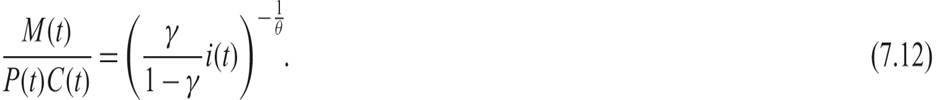
For given aggregate real consumption and nominal interest rates, the level of the nominal money supply determines the level of prices. From (7.12), it follows that

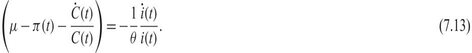
Thus, from (7.13), inflation is determined to be

For a given rate of growth in private consumption and fixed nominal interest rates, the inflation rate π(t) is determined by the rate of growth of the money supply.

Equation (7.15) is the basis of the monetary approach to the determination of inflation. In the long run, inflation is determined by the difference between the growth rate of the money supply and the long-run growth rate of aggregate output and consumption.

7.1.6 The Euler Equation for Consumption

Turning now to the first-order conditions for consumption, from (7.6) and (7.8), it follows that

which is the standard Euler equation for consumption in a representative household model. In this monetary model, it does not differ from the corresponding equation in a real model, such as the one examined in chapter 4.

The real money balances and the nominal interest rate do not appear in (7.16) because of the assumption of additively separable preferences of the household for consumption and real money balances. With additively separable preferences, the marginal utility of consumption in (7.6) does not depend on real money balances or the determinants of their demand (such as the nominal interest rate).

It is straightforward to show that without additively separable preferences, the marginal utility of consumption in (7.6) depends on real money balances as well, and (7.16) does not generally follow.

For example, consider a nonadditively separable CES instantaneous utility function of the form

where σ is the elasticity of substitution between consumption and real money balances. The first-order condition (7.6) would then take the form

With an elasticity of substitution σ different from unity (i.e., nonadditively separable preferences), the marginal utility of consumption depends on real money balances as well.

In any case, in what follows, we shall continue assuming additively separable preferences between consumption and real money balances, mainly for reasons of analytical simplicity. In this case, (7.16) holds. From (7.16), the evolution of aggregate consumption C and consumption per efficiency unit of labor c are determined by

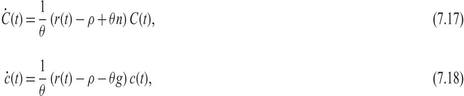
where g is the rate of exogenous technical progress.

From (7.17) and (7.18), the rate of growth of aggregate consumption (or consumption per efficiency unit of labor) only depends on real variables and not the money supply or its rate of growth.

7.2