Problems of Infinity

Let us discuss the following abstract general equilibrium economy introduced by Karl Shell. We will see that the baseline overlapping generations model of Samuelson and Diamond is very closely related to this abstract economy.

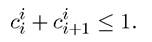
Consider the following static economy with a countably infinite number of households, each denoted by i ∈ N, and a countably infinite number of commodities, denoted by j ∈ N. Assume that all households behave competitively (alternatively, we can assume that there are M households of each type, and M is a large number). Household i has preferences given by:

where cj denotes the consumption of the jth type of commodity by household i. These preferences imply that household i enjoys the consumption of the commodity with the same index as its own index and the next indexed commodity (i.e., if an individual’s index is 3, she only derives utility from the consumption of goods indexed 3 and 4, etc.).

The endowment vector ω of the economy is as follows: each household has one unit endowment of the commodity with the same index as its index. Let us choose the price of the first commodity as the numeraire, i.e., po = 1.

The following proposition characterizes a competitive equilibrium. Exercise 9.1 asks you to prove that this is the unique competitive equilibrium in this economy.

Proposition 9.1. In the above-described economy, the price vector _ such that pj = 1 for all j ∈ N is a competitive equilibrium price vector and induces an equilibrium with no trade, denoted by x.

Proof. At p, each household has income equal to 1. Therefore, the budget constraint of household i can be written as

This implies that consuming own endowment is optimal for each household, establishing that the price vector p and no trade, x, constitute a competitive equilibrium.

However, the competitive equilibrium in Proposition 9.1 is not Pareto optimal. To see this, consider the following alternative allocation,Household i = 0 consumes one unit of good j = 0 and one unit of good j = 1, and household i > 0 consumes one unit of good i + 1. In other words, household i = 0 consumes its own endowment and that of household 1, while all other households, indexed i > 0, consume the endowment of than neighboring household, i + 1. In this allocation, all households with i > 0 are as well off as in the competitive equilibrium (p, x), and individual i = 0 is strictly better-off. This establishes:

Proposition 9.2. In the above-described economy, the competitive equilibrium at (p, ^x) is not Pareto optimal.

So why does the First Welfare Theorem not apply in this economy? Recall that the first version of this theorem, Theorem 5.5, was stated under the assumption of a finite number of commodities, whereas we have an infinite number of commodities here. Clearly, the source of the problem must be related to the infinite number of commodities. The extended version of the First Welfare Theorem, Theorem 5.6, covers the case with an infinite number of commodities, but only under the assumption that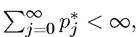where pj refers to the price

of commodity j in the competitive equilibrium in question. It can be immediately verified that this assumption is not satisfied in the current example, since the competitive equilibrium in question featuresAs discussed in Chapter 5,

when the sum of prices is equal to infinity, there can be feasible allocations for the economy as a whole that Pareto dominate the competitive equilibrium. The economy discussed here gives a simple example where this happens.

If the failure of the First Welfare Theorem were a specific feature of this abstract (perhaps artificial) economy, it would not have been of great interest to us. However, this abstract economy is very similar (in fact “isomorphic”) to the baseline overlapping generations model. Therefore, the source of inefficiency (Pareto suboptimality of the competitive equilibrium) in this economy will be the source of potential inefficiencies in the baseline overlapping genera­tions model.

It is also useful to recall that, in contrast to Theorem 5.6, the Second Welfare Theorem, Theorem 5.7, did not make use of the assumption that ______________ 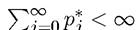even when the number

of commodities was infinite. Instead, this theorem made use of the convexity of preferences, consumption sets and production possibilities sets. So one might conjecture that in this model, which is clearly an exchange economy with convex preferences and convex consumption sets, Pareto optima must be decentralizable by some redistribution of endowments (even though competitive equilibrium may be Pareto suboptimal). This is in fact true, and the following proposition shows how the Pareto optimal allocation x described above can be decentralized as a competitive equilibrium:

PROPOSITION 9.3. In the above-described economy, there exists a reallocation of the en­dowment vector ω to ω, and an associated competitive equilibriumthat is Pareto opti­mal where x is as described above, andis such that pj = 1 for all j ∈ N.

Proof. Consider the following reallocation of the endowment vector ω: the endowment of household i ≥ 1 is given to household i — 1. Consequently, at the new endowment vector ω, household i = 0 has one unit of good j = 0 and one unit of good j = 1, while all other 347

households i have one unit of good i + 1. At the price vector p, household 0 has a budget set thus chooses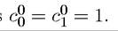All other households have budget sets given by

thus it is optimal for each household i > 0 to consume one unit of the goodwhich is

within its budget set and gives as high utility as any other allocation within his budget set, establishing that x is a competitive equilibrium. ?

9.2.