The Baseline Overlapping Generations Model
We now discuss the baseline two-period overlapping generation economy.
9.2.1. Demographics, Preferences and Technology. In this economy, time is discrete and runs to infinity.
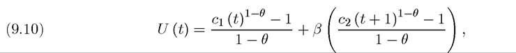
Each individual lives for two periods. For example, all individuals born at time t live for dates t and t + 1. For now let us assume a general (separable) utility function for individuals born at date t, of the form
where u : satisfies the conditions in Assumption 3, ci (t) denotes the consumption of
the individual born at time t when young (which is at date t), and c2 (t + 1) is the individual’s consumption when old (at date t + 1). Also β ∈ (0,1) is the discount factor.
Factor markets are competitive. Individuals can only work in the first period of their lives and supply one unit of labor inelastically, earning the equilibrium wage rate w (t).
Let us also assume that there is exponential population growth, so that total population is

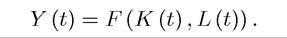
The production side of the economy is the same as before, characterized by a set of competitive firms, and is represented by a standard constant returns to scale aggregate production function, satisfying Assumptions 1 and 2;
To simplify the analysis let us assume that δ = 1,so that capital fully depreciates after use (see Exercise 9.3). Thus, again defining the (gross) rate of return to saving, which
equals the rental rate of capital, is given by 
where f (k) ? F (k, 1) is the standard per capita production function.
As usual, the wage rate is(9.4) 
9.2.2. Consumption Decisions. Let us start with the individual consumption decisions. Savings by an individual of generation t, s (t), is determined as a solution to the following maximization problem
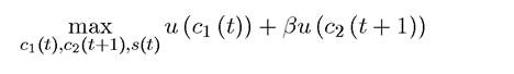
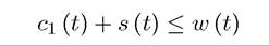
subject to
and
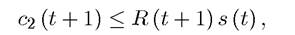
where we are using the convention that old individuals rent their savings of time t as capital to firms at time t + 1, so they receive the gross rate of return R (t +1) = 1+ r (t +1) (we use R instead of 1 + r throughout to simplify notation). The second constraint incorporates the notion that individuals will only spend money on their own end of life consumption (since there is no altruism or bequest motive). There is no need to introduce the additional constraint that s (t) ≥ 0, since negative savings would violate the second-period budget constraint (given that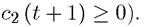
Since the utility function u (∙) is strictly increasing (Assumption 3), both constraints will hold as equalities. Therefore, the first-order condition for a maximum can be written in the familiar form of the consumption Euler equation (for the discrete time problem, recall Chapter 6),
(9.5) 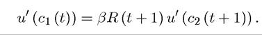
Moreover, since the problem of each individual is strictly concave, this Euler equation is sufficient to characterize an optimal consumption path given market prices.
Solving this equations for consumption and thus for savings, we obtain the following implicit function that determines savings per person as
(9.6) 
where s : is strictly increasing in its first argument and may be increasing or
decreasing in its second argument (see Exercise 9.4).
Total savings in the economy will be equal to
349
where L (t) denotes the size of generation t, who are saving for time t + 1. Since capital depreciates fully after use and all new savings are invested in the only productive asset of the economy, capital, the law of motion of the capital stock is given by
(9.7) K (t + 1) = L (t) s (w (t),R (t +1)).
9.2.3. Equilibrium. A competitive equilibrium in the overlapping generations economy can be defined as follows:
Definition 9.1. A competitive equilibrium can be represented by a sequence of aggregate capital stocks, individual consumption and factor prices, 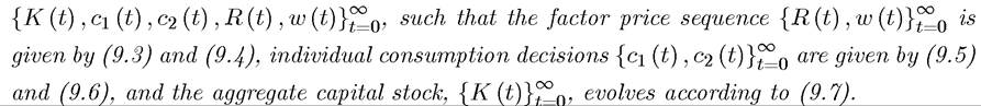
A steady-state equilibrium is defined in the usual fashion, as an equilibrium in which the capital-labor ratio k ? K/L is constant.
To characterize the equilibrium, divide (9.7) by labor supply at time t + 1, L(t + 1) = (1 + n) L (t), to obtain the capital-labor ratio as
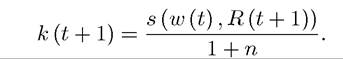
Now substituting for R (t + 1) and w (t) from (9.3) and (9.4), we obtain

as the fundamental law of motion of the overlapping generations economy. A steady state is given by a solution to this equation such that k (t + 1) = k (t) = k*, i.e.,

Since the savings function s (∙, ∙) can take any form, the difference equation (9.8) can lead to quite complicated dynamics, and multiple steady states are possible. The next figure shows some potential forms that equation (9.8) can take. The figure illustrates that the overlapping generations model can lead to a unique stable equilibrium, to multiple equilibria, or to an equilibrium with zero capital stock.
In other words, without putting more structure on utility and/or production functions, the model makes few predictions.9.2.4. Restrictions on Utility and Production Functions. In this subsection, we characterize the steady-state equilibrium and transition dynamics when further assumptions are imposed on the utility and production functions. In particular, let us suppose that the utility functions take the familiar CRRA form:
350
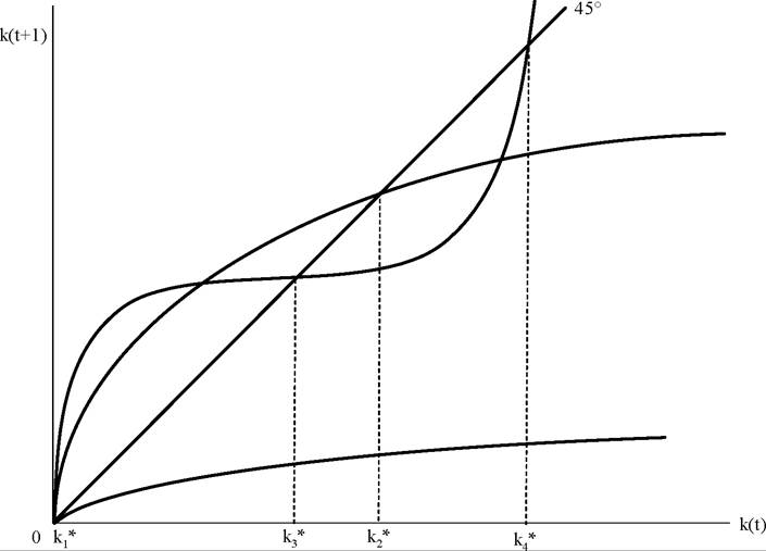
Figure 9.1. Various types of steady-state equilibria in the baseline overlapping generations model.
where θ > 0 and β ∈ (0,1). Furthermore, assume that technology is Cobb-Douglas, so that
The rest of the environment is as described above. The CRRA utility simplifies the first-order condition for consumer optimization and implies
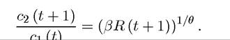
Once again, this expression is the discrete-time consumption Euler equation from Chapter 6, now for the CRRA utility function. This Euler equation can be alternatively expressed in terms of savings as

which gives the following equation for the saving rate:
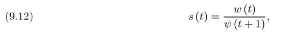
where 
which ensures that savings are always less than earnings. The impact of factor prices on savings is summarized by the following and derivatives:
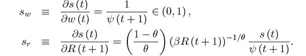
Since ψ (t + 1) > 1, we also have that 0 < sw < 1.
Moreover, in this case sr > 0 if θ < 1, sr < 0 if θ > 1, and sr = 0 if θ = 1. The relationship between the rate of return on savings and the level of savings reflects the counteracting influences of income and substitution effects. The case of θ = 1 (log preferences) is of special importance and is often used in many applied models. This special case is sufficiently common that it may deserve to be called the canonical overlapping generations model and will be analyzed separately in the next section.In the current somewhat more general context, equation (9.8) implies
(9.13) 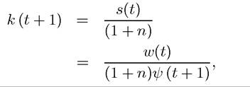
or more explicitly,
(9.14) 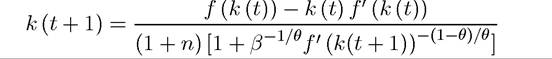
The steady state then involves a solution to the following implicit equation:
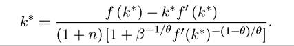
Now using the Cobb-Douglas formula, we have that the steady state is the solution to the equation
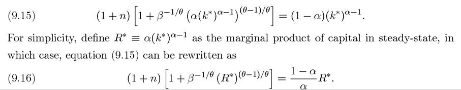
The steady-state value of R*, and thus k*, can now be determined from equation (9.16), which always has a unique solution. We can next investigate the stability of this steady state. To do this, substitute for the Cobb-Douglas production function in (9.14) to obtain

Using (9.17), we can establish the following proposition can be proved:[XXI]
Proposition 9.4. In the overlapping-generations model with two-period lived households, Cobb-Douglas technology and CRRA preferences, there exists a unique steady-state equilibrium with the capital-labor ratio k* given by (9.15) and as long as θ ≥ 1, this steady-state equilibrium is globally stable for all k (0) > 0.
Proof. See Exercise 9.5 ?
In this particular (well-behaved) case, equilibrium dynamics are very similar to the basic Solow model, and are shown in Figure 9.2, which is specifically drawn for the canonical overlapping generations model of the next section. The figure shows that convergence to the unique steady-state capital-labor ratio, k*, is monotonic. In particular, starting with an initial capital-labor ratio k (0) < ę *, the overlapping generations economy steadily accumulates more capital and converge to k*. Starting with k0 (0) > ę *, the equilibrium involves lower and lower levels of capital-labor ratio, ultimately converging to k*.
9.3.