A Quantitative Evaluation
As a final exercise, let us investigate whether the quantitative implications of the neoclassical growth model are reasonable. For this purpose, consider a world consisting of a collection J of closed neoclassical economies (with all the caveats of ignoring technological, trade and financial linkages across countries, already discussed in Chapter 3; see also Chapter 19).
Suppose that each country j ∈ J admits a representative household with identical preferences, given by
Let us assume that there is no population growth, so that Cj is both total or per capita consumption. Equation (8.38) imposes that all countries have the same discount rate ρ (see Exercise 8.16).
All countries also have access to the same production technology given by the Cobb- Douglas production function
(8.39) 
with Hj representing the exogenously given stock of effective labor (human capital). The accumulation equation is
The only difference across countries is in the budget constraint for the representative household, which takes the form
(8.40) 
where Tj is the tax on investment. This tax varies across countries, for example because of policies or differences in institutions/property rights enforcement. Notice that is also the relative price of investment goods (relative to consumption goods): one unit of consumption goods can only be transformed into
 units of investment goods.
Note that the right-hand side variable of (8.40) is still Yj, which implicitly assumes that TjIj is wasted, rather than simply redistributed to some other agents in the economy. This is without any major consequence, since, as noted in Theorem 5.2 above, CRRA preferences as in (8.38) have the nice feature that they can be exactly aggregated across individuals, so we do not have to worry about the distribution of income in the economy.
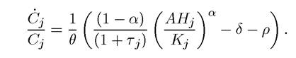
The competitive equilibrium can be characterized as the solution to the maximization of (8.38) subject to (8.40) and the capital accumulation equation.
With the same steps as above, the Euler equation of the representative household is
Consider the steady state. Because A is assumed to be constant, the steady state corresponds to This immediately implies that
id="Picutre 1026" class="lazyload" data-src="/files/uch_group77/uch_pgroup317/uch_uch7364/image/image1024.jpg">
So countries with higher taxes on investment will have a lower capital stock in steady state. Equivalently, they will also have lower capital per worker, or a lower capital output ratio (using (8.39) the capital output ratio is simply
333
Now substituting this into (8.39), and comparing two countries with different taxes (but the same human capital), we obtain the relative incomes as
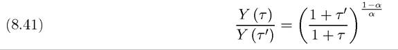
So countries that tax investment, either directly or indirectly, at a higher rate will be p oorer. The advantage of using the neoclassical growth model for quantitative evaluation relative to the Solow growth model is that the extent to which different types of distortions (here captured by the tax rates on investment) will affect income and capital accumulation is determined endogenously.
In contrast, in the Solow growth model, what matters is the saving rate, so we would need other evidence to link taxes or distortions to savings (or to other determinants of income per capita such as technology).How large will be the effects of tax distortions captured by equation (8.41)? Put differently, can the neoclassical growth model combined with policy differences account for quantitatively large cross-country income differences?
The advantage of the current approach is its parsimony. As equation (8.41) shows, only differences in τ across countries and the value of the parameter α matter for this comparison. Recall also that a plausible value for α is 2/3, since this is the share of labor income in national product which, with Cobb-Douglas production function, is equal to α, so this parameter can be easily mapped to data.
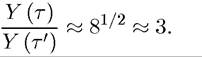
Where can we obtain estimates of differences in τ's across countries? There is no obvious answer to this question. A popular approach in the literature is to obtain estimates of τ from the relative price of investment goods (as compared to consumption goods), motivated by the fact that in equation (8.40) τ corresponds to a distortion directly affecting investment expenditures. Therefore, we may expect τ to have an effect on the market price of investment goods. Data from the Penn World tables suggest that there is a large amount of variation in the relative price of investment goods. For example, countries with the highest relative price of investment goods have relative prices almost eight times as high as countries with the lowest relative price.
Then, using α = 2/3, equation (8.41) implies that the income gap between two such countries should be approximately threefolds:
Therefore, differences in capital-output ratios or capital-labor ratios caused by taxes or tax-type distortions, even by very large differences in taxes or distortions, are unlikely to account for the large differences in income per capita that we observe in practice.
This is of course not surprising and parallels our discussion of the Mankiw-Romer-Weil approach in Chapter 3. In particular, recall that the discussion in Chapter 3 showed that differences in income per capita across countries are unlikely to be accounted for by differences in capital per worker alone. Instead, to explain such large differences in income per capita across countries, we need sizable differences in the efficiency with which these factors are used. Such differences do not feature in this model. Therefore, the simplest neoclassical model does not generate sufficient differences in capital-labor ratios to explain cross-country income differences.Nevertheless, many economists have tried (and still try) to use versions of the neoclassical model to go further. The motivation is simple. If instead of using α = 2/3, we take α = 1 /3 from the same ratio of distortions, we obtain
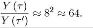
Therefore, if there is any way of increasing the responsiveness of capital or other factors to distortions, the predicted differences across countries can be made much larger. How could we have a model in which α = 1 /3? Such a model must have additional accumulated factors, while still keeping the share of labor income in national product roughly around 2/3. One possibility might be to include human capital (see Chapter 10 below). Nevertheless, the discussion in Chapter 3 showed that human capital differences appear to be insufficient to explain much of the income per capita differences across countries. Another possibility is to introduce other types of capital or perhaps technology that responds to distortions in the same way as capital. While these are all logically possible, a serious analysis of these issues requires models of endogenous technology, which will be our focus in the next part of the book.
8.10.