Real-Wage Rigidity

Because Keynesian analysis and policy prescriptions depend so greatly on the ^y. assumption that wages and prices do not move rapidly to clear markets, we begin

by discussing in some detail the possible economic reasons for slow or incomplete

adjustment.

we look at the slow adjustment of prices.

The main reason that Keynesians bring wage rigidity into their analysis is their dissatisfaction with the classical explanation of unemployment. Recall that classicals believe that most unemployment, including the increases in unemployment that occur during recessions, arises from mismatches between workers and jobs (frictional or structural unemployment). Keynesians don't dispute that mismatch is a major source of unemployment, but they are skeptical that it explains all unemployment.

Keynesians are particularly unwilling to accept the classical idea that reces­sions are periods of increased mismatch between workers and jobs. If higher unem­ployment during downturns reflected increased mismatch, Keynesians argue, recessions should be periods of particularly active search by workers for jobs and by firms for new employees. However, surveys suggest that unemployed workers spend relatively little time searching for work (many are simply waiting, hoping to be recalled to their old jobs), and help-wanted advertising and vacancy postings by firms fall rather than rise during recessions. Rather than times of increased worker­job mismatch, Keynesians believe that recessions are periods of generally low demand for both output and workers throughout the economy.

To explain the existence of unemployment without relying solely on worker­job mismatch, Keynesians argue for rejecting the classical assumption that real wages adjust relatively quickly to equate the quantities of labor supplied and demanded.

Some Reasons for Real-Wage Rigidity

For a rigid real wage to be the source of unemployment, the real wage that firms are paying must be higher than the market-clearing real wage, at which quantities of labor supplied and demanded are equal. But if the real wage is higher than nec­essary to attract workers, why don't firms save labor costs by simply reducing the wage that they pay, as suggested by the classical analysis?

Various explanations have been offered for why real wages might be rigid, even in the face of an excess supply of labor. One possibility is that there are legal and institutional factors that keep wages high, such as the minimum-wage law and union contracts. However, most U.S. workers are neither union members (less than 11% of workers were union members in 2017) nor minimum-wage earners

(about 2.3% of all hourly paid workers in 2017), so these barriers to wage cutting can't be the main reason for real-wage rigidity.^[191] Furthermore, the minimum wage in the United States is specified in nominal terms so that workers who are paid the minimum wage would have rigid nominal wages rather than rigid real wages. (Union contracts may help explain real-wage rigidity in Western European and other countries in which a higher proportion of workers are unionized.)

Another explanation for why a firm might pay a higher real wage than it "has" to is that this policy might reduce the firm's turnover costs, or the costs associated with firing existing workers or hiring and training new workers. By paying a high wage, the firm can keep more of its current workers, which saves the firm the cost of hiring and training replacements.

A third reason that firms might pay real wages above market-clearing levels is that workers who are paid well may have greater incentives to work hard and effectively. If highly paid workers are more productive, the firm may profit from paying its employees well, even though it could attract all the workers it needs at a lower real wage. The idea that a worker's productivity depends on the real wage received, and that therefore firms may pay wages above the market-clearing level, is the essence of the efficiency wage model. Because this model of wage determi­nation has played a key role in Keynesian analyses and because it has several interesting aspects, we focus on it for the remainder of this section.

The Efficiency Wage Model

If workers who are better-paid are more productive, firms may gain by paying wages higher than the minimum necessary to attract workers. But why might a worker's productivity depend on the real wage received? The answer has both "carrot" and "stick" aspects.

The carrot, or positive incentive, is based on the idea that workers who feel well treated will work harder and more efficiently. George Akerlof,^[192] a Nobel laureate at the University of California at Berkeley, argued that workers who believe that their employer is treating them fairly—say, by paying higher wages than required to retain them and by not cutting wages in slack times—will in turn want to treat the employer fairly by doing a good job. Akerlof called this motivation the gift exchange motive because it's similar to the one that leads people to exchange gifts.

The stick, or threat, aspect of why a firm would pay a higher wage than neces­sary has been analyzed in an economic model called the "shirking" model of wage determination.^[193] According to the shirking model, if workers are paid only the mini­mum amount needed to attract them to particular jobs, they won't be too con­cerned about the possibility of being fired if they don't perform well.

FIGUREJ1.1

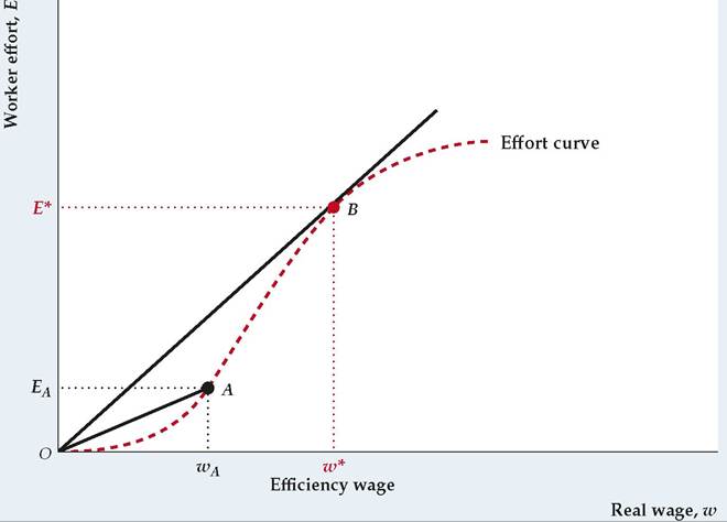
Determination of the efficiency wage

The effort curve shows the relation between worker effort, E, and the real wage workers receive, w. A higher real wage leads to more effort, but above a certain point higher wages are unable to spur effort much, so the effort curve is S-shaped. For any point on the curve, the amount of effort per dol­lar of real wage is the slope of the line from the origin to that point. At point A, effort per dollar of real wage is E_a∣w_a.

The highest level of effort per dollar of real wage is at point B, where the line from the origin is tangent to the curve. The real wage rate at B is the effi­ciency wage, w*, and the corresponding level of effort is E*.

workers aren't much happier with jobs than without jobs. In this case workers will be more inclined to take it easy at work and shirk their duties, and employers will have to bear the cost either of the shirking or of paying supervisors to make sure that the work gets done. In contrast, workers receiving higher wages will place a greater value on keeping their jobs (it's not that easy to find other jobs as good) and will work hard to avoid being fired for shirking.

The gift exchange idea and the shirking model both imply that workers' effort on the job depends on the real wages they receive. Graphically, the relationship between the real wage and the level of effort is shown by the effort curve in Figure 11.1. The real wage, w, is measured along the horizontal axis, and the level of effort, E, is measured along the vertical axis. The effort curve passes through points O, A, and B. When real wages are higher, workers choose to work harder, for either carrot or stick reasons; therefore the effort curve slopes upward. We assume that the effort curve is S-shaped.

Wage Determination in the Efficiency Wage Model

The effort curve shows that effort depends on the real wage, but what determines the real wage? To make as much profit as possible, firms will choose the level of the real wage that gets the most effort from workers for each dollar of real wages paid. The amount of effort per dollar of real wages equals the amount of effort, E, divided by the real wage, w. The ratio of E to w can be found graphically from Fig. 11.1. Consider, for

example, point A on the effort curve, at which the real wage w_A induces workers to supply effort E_a. The slope of the line from the origin to A equals the height of the curve at point A, E_a, divided by the horizontal distance, w_A. Thus the slope of the line from the origin to A equals the amount of effort per dollar of real wages at A.

The real wage that achieves the highest effort per dollar of wages is at point B. The slope of the line from the origin to B, which is the amount of effort per dollar of real wage at B, is greater than the slope of the line from the origin to any other point on the curve. In general, to locate the real wage that maximizes effort per dollar of real wage, we draw a line from the origin tangent to the effort curve; the real wage at the tangency point maximizes effort per dollar of real wage. We call the real wage that maximizes effort or efficiency per dollar of real wages the efficiency wage. In Fig. 11.1 the efficiency wage is w*, and the corresponding level of effort is E*.

The efficiency wage theory helps explain real-wage rigidity.

Employment and Unemployment in the Efficiency Wage Model

According to the efficiency wage theory, the real wage is rigid at the level that maximizes effort per dollar of wages paid. We now consider how the levels of employment and unemployment in the labor market are determined.

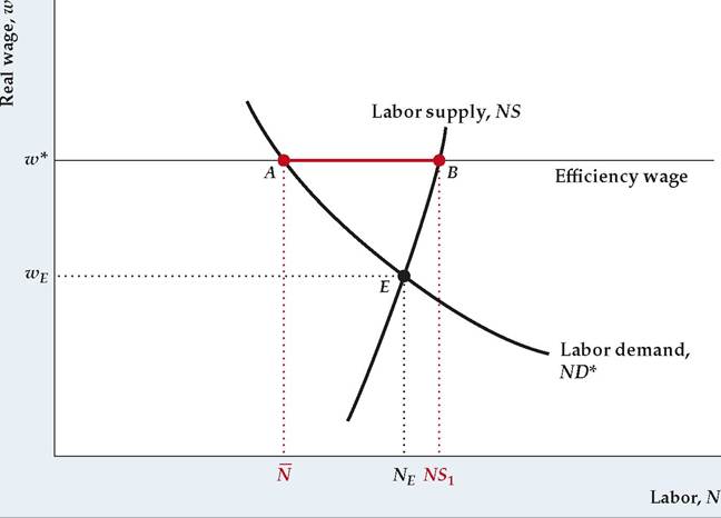
The workings of the labor market when there is an efficiency wage are shown in Figure 11.2. The efficiency wage, w*, is indicated by a horizontal line. Because the efficiency wage is determined solely by the effort curve, for the purpose of analyz­ing the labor market we can take w* to be fixed. Similarly, we can take the level of effort, E*, induced by the efficiency wage, w*, as fixed at this stage of the analysis.

The upward-sloping curve is the standard labor supply curve, NS. As in the classical model, this curve shows the number of hours of work that people would like to supply at each level of the real wage.^[194]

The downward-sloping curve is the demand curve for labor in the efficiency wage model. Recall from Chapter 3 that the amount of labor demanded by a firm depends on the marginal product of labor, or MPN. Specifically, the labor demand curve is identical to the MPN curve, which in turn relates the marginal product of labor, MPN, to the quantity of labor input, N, being used. The MPN curve—and hence the labor demand curve—slopes down because of the diminishing marginal productivity of labor.

In the classical model, the marginal product of labor depends only on the pro­duction function and the capital stock. A complication of the efficiency wage model is that the amount of output produced by an extra worker (or hour of work) also depends on the worker's effort. Fortunately, as we noted, the efficiency wage, w*, and the effort level induced by that wage, E*, are fixed at this stage of the analysis. Thus the labor demand curve in Fig. 11.2, ND*, reflects the marginal product of labor when worker effort is held fixed at E*. As in the classical case, an increase in productivity or in the capital stock shifts the labor demand curve, ND*,

FIGUREJ1.2

Excess supply of labor in the efficiency wage model

When the efficiency wage, w*, is paid, the firm's demand for labor is N, represented by point A. However, the amount of labor that workers want to supply at a real wage of w* is NS₁. The excess supply of labor equals distance

AB. We assume that the efficiency wage, w*, is higher than the market­clearing wage, w_E, that would prevail if the sup­ply of labor equaled the demand for labor at point E.

to the right. In addition, any change in the effort curve that leads to an increase in the optimal level of effort E* would raise the MPN, and the labor demand curve, ND*, again would shift to the right.

Now we can put the elements of Fig. 11.2 together to show how employment is determined. Point A on the labor demand curve, ND*, indicates that, when the real wage is fixed at w*, firms want to employ N hours of labor. Point B on the labor supply curve indicates that, when the real wage is fixed at w*, workers want to supply NS₁ hours of labor, which is greater than the amount demanded by firms. At the efficiency wage, the quantity of labor supplied is greater than the quantity demanded,^[195] so the level of employment is determined by the labor demand of firms and hence equals N. The demand-determined level of employ­ment is labeled N because it represents the full-employment level of employment for this model; that is, N is the level of employment reached after full adjustment of wages and prices. (Note that the value of N in the efficiency wage model differs from the full-employment level of employment in the classical model of the labor market, which would correspond to N_e in Fig. 11.2.) Because the efficiency wage is rigid at w*, in the absence of shocks the level of employment in this economy remains at N indefinitely.

Perhaps the most interesting aspect of Fig. 11.2 is that it provides a new expla­nation of unemployment. It shows that, even when wages have adjusted as much as they are going to and the economy is technically at "full employment," an excess supply of labor, NS₁ — N, remains.^[196]

Why don't the unemployed bid down the real wage and thus gain employ­ment, as they would in the classical model of the labor market? Unlike the classi­cal case, in a labor market with an efficiency wage the real wage can't be bid down by people offering to work at lower wages because employers won't hire them. Employers know that people working at lower wages will not put out as much effort per dollar of real wages as workers receiving the higher efficiency wage. Thus the excess supply of labor shown in Fig. 11.2 will persist indefinitely. The efficiency wage model thus implies that unemployment will exist even if there is no mismatch between jobs and workers.

The efficiency wage model is an interesting theory of real wages and unem­ployment. But does it explain actual behavior? "In Touch with Data and Research: Henry Ford's Efficiency Wage," interprets a famous episode in labor history in terms of efficiency wage theory. In addition to this anecdotal evidence, studies of wages and employment in various firms and industries provide some support for the efficiency wage model. For example, Peter Cappelli of the University of Pennsylvania and Keith Chauvin of the University of Kansas^[197] found that, consis­tent with one aspect of the theory, plants that paid higher wages to workers expe­rienced less shirking, measured by the number of workers fired for disciplinary reasons. Also, research by Michelle Alexopoulos and Jon Cohen of the University of Toronto^[198] showed that when wages became compressed in Sweden in the 1970s, workers' effort declined dramatically.

A criticism of the efficiency wage model presented here is that it predicts that the real wage is literally fixed (for no change in the effort curve). Of course, this result is too extreme because the real wage does change over time (and over the business cycle, as demonstrated in Chapter 8). However, the basic model can be extended to allow for changes in the effort curve that bring changes in the effi­ciency wage over time. For example, a reasonable assumption would be that workers are more concerned about losing their jobs during recessions, when find­ing a new job is more difficult, than during booms. Under this assumption, the real wage necessary to obtain any specific level of effort will be lower during recessions; hence the efficiency wage paid in recessions also may be lower. This extension may help the efficiency wage model match the business cycle fact that real wages are lower in recessions than in booms (procyclical real wages).

Efficiency Wages and the FE Line

In the Keynesian version of the IS-LM model, as in the classical version, the FE line is vertical, at a level of output that equals the full-employment level of output, Y. If we assume that employers pay efficiency wages, full-employment output, Y, in turn is the output produced when employment is at the full-employment level of employment, N, as shown in Fig. 11.2, and the level of worker effort is E*.

In Touch with Data and Research

Henry Ford's Efficiency Wage

During 1908-1914 Henry Ford instituted at Ford Motor Company a radically new way of producing automobiles.^[199] Prior to Ford's innovations, automobile compo­nents weren't produced to uniform specifications. Instead, cars had to be assem­bled one by one by skilled craftsmen, who could make the parts fit even if sizes or shapes were off by fractions of an inch. Ford introduced a system of assemblyline production in which a standardized product, the Model T automobile, was pro­duced from precisely made, interchangeable components. The production process also was broken into numerous small, simple steps, replacing the skilled craftsmen who had built cars from start to finish with unskilled workers who performed only a few operations over and over.

The high speed at which Ford ran the assembly line and the repetitiveness of the work were hard on the workers. As one laborer said, "If I keep putting on Nut No. 86 for about 86 more days, I will be Nut No. 86 in the Pontiac bughouse."^[200] As a result, worker turnover was high, with the typical worker lasting only a few months on the job. Absenteeism also was high—about 10% on any given day— and morale was low. Worker slowdowns and even sabotage occurred.

In January 1914 Ford announced that the company would begin paying $5 a day to workers who met certain criteria, one being that the worker had been with the company at least six months. Five dollars a day was more than double the nor­mal wage for production workers at the time. Although the motivation for Ford's announcement has been debated, its effect was stunning: Thousands of workers lined up outside the plant, hoping for jobs. Within the plant the number of people quitting dropped by 87%, absenteeism dropped by 75%, and productivity rose by 30% or more. The productivity increases helped increase Ford's profits, despite the higher wage bill and a cut in the price of a Model T.

Many results of Ford's $5 day can be predicted by the efficiency wage model, including improved efficiency and higher profits. As other automakers adopted Ford's technological innovations, they also adopted his wage policies. By 1928, before unions were important in the industry, auto industry wages were almost 40% higher than those in the rest of manufacturing.

⁹The source for this box is Daniel M. G. Raff and Lawrence H. Summers, "Did Henry Ford Pay Efficiency Wages?" Journal of Labor Economics, October 1987, pp. S57-S86.

¹⁰This quote is originally from Stephen Meyer, The Five-Dollar Day: Labor Management and Social Control in the Ford Motor Company, 1908-1921, Albany: State University of New York Press, 1981. product of labor at any given level of employment, a drop in productivity reduces the demand for labor at any fixed real wage. With the real wage fixed at w*, the full-employment level of employment, N, falls. Second, a drop in productivity reduces the amount of output that can be produced with any particular amount of capital, labor, and effort.

11.2