Price Stickiness

Describe the causes and effects of price stickiness according to the Keynesian model.

The rigidity created by efficiency wages is a real rigidity in that the real wage, rather than the nominal wage, remains fixed.

We explained in Section 11.1 that Keynesians introduced real-wage rigidity because of their dissatisfaction with the classical explanation of unemployment. Similarly, the assumption of price stickiness addresses what Keynesians believe is another significant weakness of the basic classical model: the classical prediction that money is neutral.

Recall that, in the basic classical model without misperceptions, the assump­tion that wages and prices adjust quickly implies that money is neutral. If money is neutral, an increase or decrease in the money supply changes the price level by the same proportion but has no effect on real variables, such as output, employ­ment, or the real interest rate. However, recall also that empirical studies—including analyses of historical episodes—have led most economists to conclude that money probably is not neutral in the real world.

One approach to accounting for monetary nonneutrality (pursued in Chapter 10) is to extend the classical model by assuming that workers and firms have imper­fect information about the current price level (the misperceptions theory). However, Keynesians favor an alternative explanation of monetary nonneutrality: Prices are sticky; that is, they don't adjust quickly. If prices are sticky, the price level can't adjust immediately to offset changes in the money supply, and money isn't neutral.

Although we focus on nominal-price rigidity in this section, a long Keynesian tra­dition emphasizes nominal-wage rigidity instead of nominal-price rigidity. We discuss an alternative version of the Keynesian model that rests on the assumption of nominal- wage rigidity in Appendix 11.A. This alternative model has similar implications to the Keynesian model with price rigidity—in particular, that money is not neutral.

Sources of Price Stickiness: Monopolistic Competition and Menu Costs

To say that price stickiness gives rise to monetary nonneutrality doesn't com­pletely explain nonneutrality because it raises another question: Why are prices sticky? The Keynesian explanation for the existence of price rigidity relies on two main ideas: (1) Most firms actively set the prices of their products rather than tak­ing the prices of their output as given by the market; and (2) when firms change prices, they incur a cost, known as a menu cost.

Monopolistic Competition. Talking about price stickiness in a highly com­petitive, organized market—such as the market for corn or the stock exchange— wouldn't make much sense. In these markets, prices adjust rapidly to reflect changes in supply or demand. Principal reasons for price flexibility in these competitive, highly organized markets include standardization of the product being traded (one bushel of corn of a certain grade, or one share of Microsoft stock, is much like any other) and the large number of actual or potential market participants. These two factors make it worthwhile to organize a centralized market (such as the New York Stock Exchange) in which prices can react swiftly to changes in supply and demand. These same two factors also promote keen competition among buyers and sellers, which greatly reduces the ability of any individual to affect prices.

Most participants in the corn market or stock market think of themselves as price takers.

Markets having fewer participants and less standardized products than the corn or stock markets may exhibit price-setting rather than price-taking behavior. For example, consider the market for movies in a medium-sized city. This market may be fairly competitive, with many different movie theaters, each trying to attract customers from other theaters, and so on. Although the market for movies is competitive, it isn't competitive to the same degree as the corn market. If a farmer tried to raise the price of a bushel of corn by 5¢ above the market price, the farmer would sell no corn; but a movie theater that raised its ticket prices by 5¢ above its competitors' prices wouldn't lose all its customers. Because the movie the­ater 's product isn't completely standardized (it is showing a different movie than other theaters, its location is better for some people, it has different candy bars in the concession stand, a larger screen, or more comfortable seats, and so on), the theater has some price-setting discretion. It is a price setter, not a price taker.

Generally, a situation in which all buyers and sellers are price takers (such as the market for corn) is called perfect competition. In contrast, a situation in which there is some competition, but in which a smaller number of sellers and imperfect standardization of the product allow individual producers to act as price setters, is called monopolistic competition.

Perfect competition is the model underlying the classical view of price deter­mination, and, as we have said, price rigidity or stickiness is extremely unlikely in a perfectly competitive market. Keynesians agree that price rigidity wouldn't occur in a perfectly competitive market but point out that a relatively small part of the economy is perfectly competitive.

To illustrate the issues, let's return to the example of the competing movie theaters. If the market for movie tickets were perfectly competitive, how would tickets be priced? Presumably, there would be some central meeting place where buyers and sellers of tickets would congregate. Market organizers would call out "bids" (prices at which they are willing to buy) and "asks" (prices at which they are willing to sell). Prices would fluctuate continuously as new information hit the market, causing supplies and demands to change. For example, great reviews on websites such as Rotten Tomatoes and IMDb would instantly drive up the price of tickets to that movie, but news of a prospective shortage of babysitters would cause all movie ticket prices to fall.

Obviously, though, this scheme isn't how movie tickets are priced. Actual pricing by most theaters has the following three characteristics, which are also common to most price-setting markets:

1. Rather than accept the price of movies as completely determined by the mar­ket, a movie theater sets the price of tickets (or a schedule of prices), in nominal terms, and maintains the nominal price for some period of time.

2. At least within some range, the theater meets the demand that is forthcoming at the fixed nominal price. By "meets the demand" we mean that the theater will sell as many tickets as people want to buy at its fixed price, to the point that all its seats are filled.

3. The theater readjusts its price from time to time, generally when its costs or the level of demand changes significantly.

Can this type of pricing behavior maximize profits? Keynesian theory sug­gests that it can, if costs are associated with changing nominal prices, and if the market is monopolistically competitive.

Menu Costs and Price Setting. The classic example of a cost of changing prices is the cost that a restaurant faces when it has to reprint its menu to show changes in the prices of its offerings.

A potential problem with the menu cost explanation for price rigidity is that these costs seem to be rather small. How, then, can they be responsible for an amount of nominal rigidity that could have macroeconomic significance?

Here is the first point at which the monopolistic competition assumption is important. For a firm in a perfectly competitive market, getting the price "a little bit wrong" has serious consequences: The farmer who prices his corn 5ς' a bushel above the market price sells no corn. Therefore the existence of a menu cost wouldn't prevent the farmer from pricing his product at precisely the correct level. However, the demand for the output of a monopolistically competitive firm responds much less sharply to changes in its price; the movie theater doesn't lose many of its customers if its ticket price is 5ς' higher than its competitors'. Thus as long as the monopolistic competitor's price is in the right general range, the loss of profits from not getting the price exactly right isn't too great. If the loss in profits is less than the cost of changing prices—the menu costs—the firm won't change its price.

Over time, the production function and the demand curve the firm faces will undergo a variety of shocks so that eventually the profit-maximizing price for a firm may be significantly different from the preset price. When the profits lost by having the "wrong" price clearly exceed the cost of changing the price, the firm will change its nominal price. Thus movie theaters periodically raise their ticket and popcorn prices to reflect general inflation and other changes in market conditions.

Empirical Evidence on Price Stickiness. Several studies have examined the degree of rigidity or stickiness in actual prices.

To investigate whether firms perceive their own prices as being sticky or not, Alan Blinder^[201] of Princeton University, assisted by a team of Princeton graduate students, interviewed the managers of 200 randomly selected firms about their pricing behavior. Almost half (49.5%) of managers interviewed said that their firms changed prices once a year or less. Only 22% of the firms changed prices more than four times per year. Besides probing into pricing behavior, Blinder and his students also asked firm managers why they tend to change prices infrequently. Direct costs of changing prices (menu costs) did appear to play a role for many firms. Nevertheless, many managers stressed as a reason for price stickiness their concern that, if they changed their own prices, their competitors would not neces­sarily follow suit. Managers were particularly reluctant to be the first in their mar­ket to raise prices, fearing that they would lose customers to their rivals. For this reason, many firms reported delaying price changes until it was evident through­out the industry that changes in costs or demand made price adjustment necessary.

In another study of price stickiness Anil Kashyap,^[202] of the University of Chicago, examined the prices of twelve individual items listed in the catalogues of L.L. Bean, Orvis, and Recreational Equipment, Inc., over a 35-year period. Changing the prices listed in a new catalogue is virtually costless, yet Kashyap found that the nominal prices of many goods remained fixed in successive issues of the catalogue.

However, evidence based on a larger data set suggests that price stickiness may not be as pervasive as earlier studies indicated. In their 2004 paper, Mark Bils of the University of Rochester and Peter Klenow of Stanford University^[203] found that the average time between price changes among 350 categories of goods (whose prices were recorded by the Bureau of Labor Statistics for use in calculat­ing the Consumer Price Index) was just 4.3 months, suggesting that prices are changed much more frequently than reported by Blinder and by Kashyap. Prices of some goods and services, such as men's haircuts, taxicab fares, and newspa­pers, change very rarely and are clearly sticky. But prices of other goods and ser­vices, including food and gasoline, change very frequently.

The results by Bils and Klenow thus suggest that some prices are not too sticky, and these findings could cast doubt on the price stickiness view. Even though some prices may adjust frequently, many economists continue to use price stickiness in their models because the causes of the price changes are important. For instance, when firms run sales, they reduce their prices at the beginning of the sale and increase prices at the end of the sale. A study by Emi Nakamura and Jon Steinsson^[204] of Columbia University found that if one looks at all changes in prices, including the changes that occur during sales, the median time between price changes is about 4.6 months, which is close to the finding in Bils and Klenow. However, when Nakamura and Steinsson exclude price changes associated with sales, they find that the median length of time between price changes more than doubles to 11 months, which is consistent with stickiness in non-sales prices. Another reason that economists continue to use the assumption of price stickiness in their models is that many of the price changes are caused by shifts in demand or supply in a particular industry. For example, day-to-day news about the supply of oil causes gasoline prices to change. But the assumption about price stickiness is going to be relevant in our macroeconomic model for how prices respond to changes in mon­etary policy and how prices change to restore general equilibrium, not how they respond to supply and demand shocks in their own industry. Research by Jean Boivin of HEC-Montreal, Marc Giannoni of the Federal Reserve Bank of Dallas, and Ilian Mihov of INSEAD^[205] shows that in response to monetary policy, prices of many goods are very sticky, whereas those same prices respond quickly in response to shocks to supply and demand that affect the relative price of the good compared with other goods. Thus in our macroeconomic model, the assumption of sticky prices is a useful one, even in the face of the Bils and Klenow evidence.

Meeting the Demand at the Fixed Nominal Price. When prices are sticky, firms react to changes in demand by changing the amount of production rather than by changing prices. According to Keynesians, why are firms willing to meet demand at a fixed nominal price? To answer this question, we again rely on the assumption of monopolistic competition. We've stated that a monopolistically competitive firm can raise its price some without risk of losing all its customers. The profit-maximizing strategy for a monopolistically competitive firm is to charge a price higher than its marginal cost, or the cost of producing an additional unit of output. The excess of the price over the marginal cost is the markup. For example, if a firm charges a price 15% above its marginal cost, the firm has a markup of 15%. More generally, if the firm charges a constant markup of η over marginal cost, the following markup rule describes its price:

P = ( 1 + η) MC, (11.1)

where P is the nominal price charged by the firm and MC is the nominal marginal cost.^[206]

When the firm sets its price according to Eq. (11.1), it has an idea of how many units it will sell. Now suppose that, to the firm's surprise, customers demand sev­eral more units than the firm expected to sell at that price. Will it be profitable for the firm to meet the demand at this price?

The answer is "yes." Because the price the firm receives for each extra unit exceeds its cost of producing that extra unit (its marginal cost), the firm's profits increase when it sells additional units at the fixed price. Thus as long as the mar­ginal cost remains below the fixed price of its product, the firm gladly supplies

FIGUREJ1.3

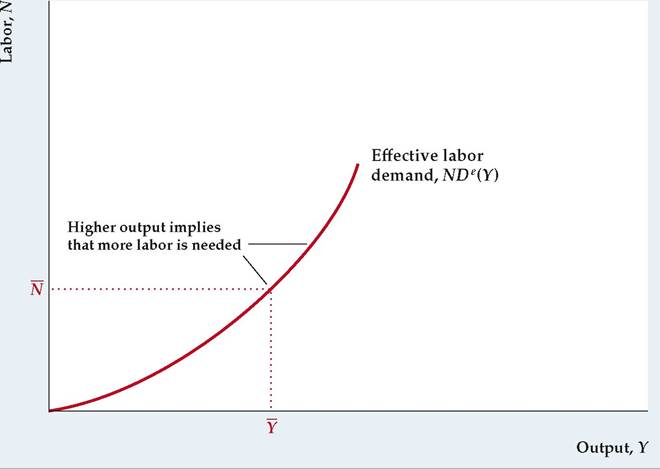
The effective labor demand curve

When a firm meets the demand for its output, it employs just the amount of labor needed to pro­duce the quantity of out­put demanded. Because more labor is required to produce more output, firms must employ more labor when the demand for output is higher.

This relationship between the amount of output demanded and the amount of labor employed is the effective labor demand curve. The effective labor demand curve is the same as the production function relating output and labor, except that labor is plot­ted on the vertical axis and output is plotted on the horizontal axis.

more units at this fixed price. Furthermore, if the firm is paying an efficiency wage, it can easily hire more workers to produce the units needed to meet the demand because there is an excess supply of labor.

The macroeconomic importance of firms' meeting demand at the fixed nomi­nal price is that the economy can produce an amount of output that is not on the full­employment line. Recall that the FE line shows the amount of output that firms would produce after complete adjustment of all wages and prices. However, with nominal-price stickiness the prices of goods do not adjust rapidly to their general equilibrium values. During the period in which prices haven't yet completely adjusted, the amount of output produced need not be on the FE line. Instead, as long as marginal cost is below the fixed price, monopolistically competitive firms will produce the level of output demanded.

Effective Labor Demand. When a firm meets the demand for its output at a specific price, it may produce a different amount of output and employ a different amount of labor than it had planned. How much labor will a firm actually employ when it meets the demand? The answer is given by the effective labor demand curve, ND^e (Y), shown in Figure 11.3. For any amount of output, Y, the effective labor demand curve indicates how much labor is needed to produce that output, with productivity, the capital stock, and effort held constant.

We already have a concept that expresses the relationship between the amount of labor used and the amount of output produced: the production func­tion. Indeed, the effective labor demand curve in Fig. 11.3 is simply a graph of the production function relating output and labor input, except that output, Y, is measured on the horizontal axis and labor, N, is measured on the vertical axis. (This reversal of the axes is convenient later.) The effective labor demand curve slopes upward from left to right because a firm needs more labor to produce more output.

We use the effective labor demand curve to determine the level of employ­ment in the Keynesian model in Section 11.3. When the economy is not on the FE line and the price level is fixed, the effective labor demand curve gives the level of employment. Then, after complete adjustment of wages and prices, the economy returns to the FE line and the level of employment is given by the labor demand curve, ND* (Fig. 11.2). After wages and prices have completely adjusted, with out­put at its full-employment level, Y, the effective labor demand curve indicates that employment equals N, as shown in Fig. 11.3.

11.3