Monetary and Fiscal Policy in the Keynesian Model

Analyze the effects Let's now consider the complete Keynesian model. Like the classical model, the of m°^netar^{y an}d Keynesian model can be expressed in terms of the IS-LM diagram or, alternatively,

in terms of the AD-AS diagram.

Monetary Policy

The main reason for introducing nominal-price stickiness into the Keynesian model was to explain monetary nonneutrality. We examine the link between price stickiness and monetary nonneutrality first in the Keynesian IS-LM framework and then in the Keynesian version of the AD-AS model.

Monetary Policy in the Keynesian IS-LM Model. The Keynesian version of the IS-LM model is quite similar to the IS-LM model discussed in Chapters 9 and 10. In particular, the IS curve and the LM curve are the same as in our earlier analyses. The FE line in the Keynesian model also is similar to the FE line used earlier. The Keynesian FE line is vertical at the full-employment level of output, Y, which in turn depends on the full-employment level of employment determined in the labor market. However, the Keynesian and classical FE lines differ in two respects. First, in the Keynesian model the full-employment level of employment is determined at the intersection of the labor demand curve and the efficiency wage line, not at the point where the quantities of labor demanded and supplied are equal, as in the classical model. Second, because labor supply doesn't affect employment in the efficiency wage model, changes in labor supply don't affect the Keynesian FE line, although changes in labor supply do affect the classical FE line. Because of price stickiness, in the Keynesian model the economy doesn't have to be in general equilibrium in the short run.

According to Keynesians, what happens to the economy in the short run if sticky prices prevent it from reaching general equilibrium? Keynesians assume that the asset market clears quickly and that the level of output is determined by aggregate demand. Thus according to Keynesians, the economy always lies at the intersection of the IS and LM curves. However, because monopolistically competi­tive firms are willing to meet the demand for goods at fixed levels of prices, out­put can differ from full-employment output and the economy may not be on the

FE line in the short run. When the economy is off the FE line, firms use just enough labor to produce the output needed to meet demand. Under the assumption that the efficiency wage is higher than the market-clearing real wage, there are always unemployed workers who want to work, and firms are able to change employ­ment as needed to meet the demand for output without changing the wage.

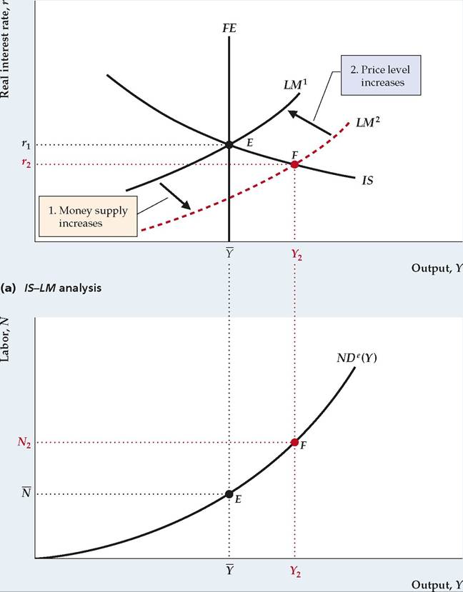
Figure 11.4 analyzes the effect of an increase in the nominal money supply in the Keynesian IS-LM model. We assume that the economy starts at its general equilibrium point, E. Recall that an increase in the money supply shifts the LM curve down and to the right, from LM¹ to LM² (Fig. 11.4a). Because an increase in

FIGURE 11.4

An increase in the money supply

(a) If we start from an initial general equilib­rium at point E, an increase in the money supply shifts the LM curve down and to the right, from LM¹ to LM²; the IS curve and the FE line remain unchanged. Because prices are fixed and firms meet the demand for output in the short run, the economy moves to point F, which is to the right of the FE line. Output rises to Y₂ and the real interest rate falls.

(b) Because firms pro­duce more output, employment rises to N 2, as shown by the effective labor demand curve.

In the long run, the price level rises in the same proportion as the money supply, the real money supply returns to its ini­tial level, and the LM curve returns to its initial position, LM 1, in (a). The economy returns to E in both (a) and (b), and money is neutral in the long run.

(b) Effective labor demand

the money supply doesn't directly affect the goods or labor markets, the IS curve and the FE line are unaffected. So far this analysis is like that of the classical model.

Unlike the classical model, however, the Keynesian model is based on the assumption that prices are temporarily fixed (because of menu costs) so that the general equilibrium at E isn't restored immediately. Instead, the short-run equilib­rium of the economy—that is, the resting point of the economy at the fixed price level—lies at the intersection of IS and LM² (point F), where output rises to Y₂ and the real interest rate falls to r₂.

Because the IS-LM intersection at point F is to the right of the FE line, aggre­gate output demanded, Y₂, is greater than the full-employment level of output, Y. Monopolistically competitive firms facing menu costs don't raise their prices in the short run, as competitive firms do. Instead they increase production to Y₂ to satisfy the higher level of demand. To increase production, firms raise employment— for example, by hiring additional workers or by having employees work over­time. The level of employment is given by the effective labor demand curve in Fig. 11.4(b). Because the level of output increases from Y to Y₂ in the short run, the level of employment increases from N to N₂.

We refer to a monetary policy that shifts the LM curve down and to the right— and thus increases output and employment—as an expansionary monetary policy, or "easy" money. Analogously, a contractionary monetary policy, or "tight" money, is a decrease in the money supply that shifts the LM curve up and to the left, decreas­ing output and employment.

Why does easy money increase output in the Keynesian model? In the Keynesian model, prices are fixed in the short run, so an increase in the nominal money supply, M, also is an increase in the real money supply, M∕P. Recall that, for holders of wealth to be willing to hold more real money, the real interest rate must fall.^[207] Finally, the lower real interest rate increases both consumption spend­ing (because saving falls) and investment spending. With more demand for their output, firms increase production and employment, taking the economy to point F in Fig. 11.4.

The rigidity of the price level isn't permanent. Eventually, firms will review and readjust their prices, allowing the economy to reach its long-run equilibrium. In the case of monetary expansion, firms find that demand for their products in the short run is greater than they had planned (aggregate output demanded, Y₂, is greater than full-employment output, Y), so eventually they raise their prices. The rise in the price level returns the real money supply to its initial level, which shifts the LM curve back to LM¹ and restores the general equilibrium at point E in Fig. 11.4(a). This adjustment process is exactly the same as in the classical model, but it proceeds more slowly.

Thus the Keynesian model predicts that money is not neutral in the short run but is neutral in the long run. In this respect the predictions of the Keynesian model are the same as those of the extended classical model with misperceptions. In the Keynesian model, short-run price stickiness prevents the economy from reaching its general equilibrium, but in the long run prices are flexible, ensuring general equilibrium.

Monetary Policy in the Keynesian AD-AS Model. We can also analyze the effect of monetary policy on real output and the price level by using the Keynesian version of the AD-AS model. In fact, we have already performed this analysis in Fig. 9.14, where we used the AD-AS model to examine the effects of a 10% increase in the nominal money supply.

The distinguishing feature that determines whether an analysis is Keynesian or classical is the speed of price adjustment. As we emphasized in Chapter 10, classical economists argue that prices adjust quickly so that the economy reaches its long-run equilibrium quickly. In the extreme version of the classical model, the long-run equilibrium is reached virtually immediately, and the short-run aggre­gate supply (SRAS) curve is irrelevant. However, in the Keynesian model, monop­olistically competitive firms that face menu costs keep their prices fixed for a while, producing the amount of output demanded at the fixed price level. This behavior is represented by a horizontal short-run aggregate supply curve such as SRAS¹ in Fig. 9.14. If we assume that firms maintain fixed prices and simply meet the demand for output for a substantial period of time, so that the departure from long-run equilibrium lasts for months or perhaps even years, the analysis illus­trated in Fig. 9.14 reflects the Keynesian approach.

Let's briefly review that analysis from an explicitly Keynesian perspective. Figure 9.14 depicts the effects of a 10% increase in the nominal money supply on an economy that is initially in both short-run and long-run equilibrium (at point E). The increase in the nominal money supply causes the AD curve to shift up from AD¹ to AD². In fact, as we explained in Chapter 9, the 10% increase in the nominal money supply shifts the AD curve up by 10% at each level of output. The initial effect of this shift in the AD curve is to move the economy to a short-run equilibrium at point F, where output is higher than its full-employment level, Y. Because of menu costs, firms don't immediately react to increased demand by raising prices, but instead increase production to meet the higher demand. Thus at point F, firms are producing more output than the amount that would maximize their profits in the absence of menu costs.

Fiscal Policy

The Keynesian model was initially developed during the Great Depression as economists struggled to explain the worldwide economic collapse and find poli­cies to help the economy return to normal. The early Keynesians stressed that fiscal policy—the government's decisions about government purchases and taxes—can significantly affect output and employment levels. Let's look at the Keynesians' conclusion that both increased government purchases and lower taxes can be used to raise output and employment.

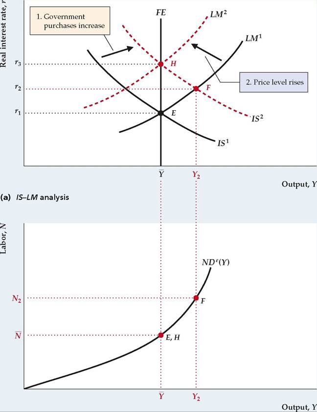
The Effect of Increased Government Purchases. The Keynesian analysis of how increased government purchases affect the economy is shown in Figure 11.5. Again, we assume that the economy starts from full employment (later we discuss what happens if the economy starts from a recession). Point E repre­sents the initial equilibrium in both (a) and (b). As before, a temporary increase in government purchases increases the demand for goods and reduces desired national saving at any level of the real interest rate, so that the IS curve shifts up and to the right, from IS¹ to IS² (see Summary table 12 in Chapter 9). In the short run, before prices can adjust, the economy moves to point F in Fig. 11.5(a), where the new IS curve, IS², and LM¹ intersect. At F both output and the real interest rate have increased. Because firms meet the higher demand at the fixed price level, employment also rises, as shown by the movement from point E to point F along the effective labor demand curve in Fig. 11.5(b). A fiscal policy change, such as this one, that shifts the IS curve up and to the right and raises output and employment is an expansionary change. Similarly, a fiscal policy change (such as a reduction in government purchases) that shifts the IS curve down and to the left and reduces output and employment is a contractionary change.

FIGURE 11.5

A temporary increase in government purchases

(a) If we start from the general equilibrium at point E, a temporary increase in government purchases reduces desired national saving and shifts the IS curve up and to the right, from IS¹ to IS². The short-run equilibrium is at point F, with output increasing to Y₂ and the real interest rate rising to r₂.

(b) As firms increase pro­duction to meet the demand, employment increases from N to N ₂, as shown by the effective labor demand curve. However, the economy doesn't remain at point F. Because aggregate out­put demanded exceeds Y in the short run, the price level increases, reducing the real money supply and shifting the LM curve up and to the left, from LM¹ to LM². In the long run, with equilib­rium at point H, output returns to Y and employ­ment returns to N, but the real interest rate rises further to r₃.

(b) Effective labor demand

In discussing the effects of increased government purchases or other types of spending, Keynesians often use the multiplier concept. The multiplier asso­ciated with any particular type of spending is the short-run change in total out­put resulting from a one-unit change in that type of spending. So, for example, if the increase in government purchases analyzed in Fig. 11.5 is AG and the resulting short-run increase in output between points E and F in Fig. 11.5 is AY, the multiplier associated with government purchases is AY/AG. Keynesians usually argue that the fiscal policy multiplier is greater than 1, so that if govern­ment purchases rise by $1 billion, output will rise by more than $1 billion. We derive an algebraic expression for the government purchases multiplier in Appendix 11.C.

Recall that the classical version of the IS-LM model also predicts that a tem­porary increase in government purchases increases output, but in a different way. The classical analysis focuses on the fact that increased government purchases require higher current or future taxes to pay for the extra spending. Higher taxes make workers (who are taxpayers) effectively poorer, which induces them to sup­ply more labor. This increase in labor supply shifts the FE line to the right and causes output to rise in the classical model. In contrast, the FE line in the Keynesian model doesn't depend on labor supply (because of efficiency wages) and thus is unaffected by the increase in government purchases. Instead, the increase in government purchases affects output by raising aggregate demand (that is, by shifting the IS-LM intersection to the right). Output increases above its full-employment level in the short run as firms satisfy extra demand at the initial price level.

The effect of increased government purchases on output in the Keynesian model lasts only as long as needed for the price level to adjust. (However, many Keynesians believe that price adjustment is sufficiently slow that this effect could be felt for several years.) In the long run, when firms adjust their prices, the LM curve moves up and to the left, from LM¹ to LM² in Fig. 11.5(a), and the economy reaches general equilibrium at point H, with output again at Y. Thus an increase in government purchases doesn't raise output in the long run.

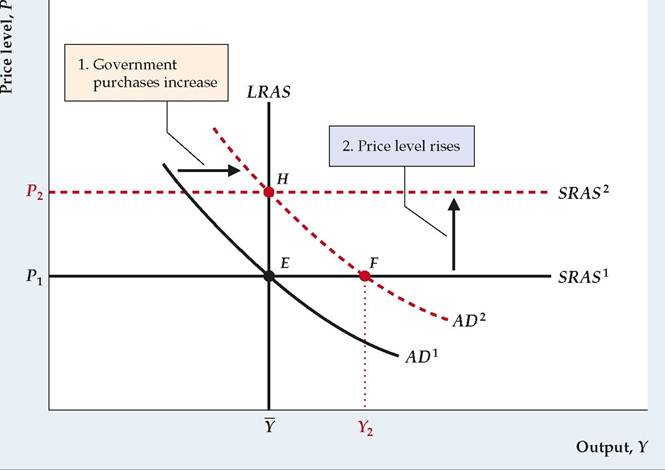
The effects of increased government purchases also appear in the Keynesian AD-AS framework (Figure 11.6). Increased government purchases shift the IS curve up and to the right and raise the aggregate demand for output at any given price level. Thus as a result of expansionary fiscal policy, the aggregate demand curve shifts to the right, from AD¹ to AD². The increase in aggregate demand raises output above Y, as shown by the shift from the initial equilibrium at point E to the short-run equilibrium at point F. At F the aggregate demand for output is greater than full-employment output, so firms eventually raise their prices. In the long run the economy reaches the full-employment general equilibrium at point H, with output again at Y and with a higher price level. These results are identical to those we obtained using the Keynesian IS-LM framework.

FIGUREJ1.6

An increase in government purchases in the Keynesian AD-AS framework

An increase in govern­ment purchases raises aggregate demand for output at any price level (see Fig. 11.5). Thus the aggregate demand curve shifts to the right, from AD¹ to AD ². In the short run the increase in aggre­gate demand increases output to Y₂ (point F) but doesn't affect the price level because prices are sticky in the short run. Because aggregate out­put demanded, Y₂, exceeds Y at F, firms eventually raise their prices. The long-run equilibrium is at H, where AD² intersects the LRAS curve. At H, out­put has returned to Y and the price level has risen from P₁ to P₂. The higher price level raises the short-run aggregate supply curve, from SRAS¹ to SRAS².

The Effect of Lower Taxes. Keynesians generally believe that, like an increase in government purchases, a lump-sum reduction in current taxes is expansionary. In other words, they expect that a tax cut will shift the IS curve up and to the right, raising output and employment in the short run. Similarly, they expect a tax increase to be contractionary, shifting the IS curve down and to the left.

Why does a tax cut affect the IS curve, according to Keynesians? The argu­ment is that if consumers receive a tax cut, they will spend part of it on increased consumption. For any output, Y, and level of government purchases, G, an increase in desired consumption arising from a tax cut will lower desired national saving, Y-C^d - G. A drop in desired saving raises the real interest rate that clears the goods market and shifts the IS curve up.^[208]

If a tax cut raises desired consumption and shifts the IS curve up, as Keynesians claim, the effects on the economy are similar to the effects of increased govern­ment purchases (Figs. 11.5 and 11.6). In the short run, a tax cut raises aggregate demand and thus output and employment at the initial price level. In the long run, after complete price adjustment, the economy returns to full employment with a higher real interest rate than in the initial general equilibrium. The only difference between the tax cut and the increase in government purchases is that, instead of raising the portion of full-employment output devoted to government purchases, a tax cut raises the portion of full-employment output devoted to consumption.

11.3