The Keynesian Theory of Business Cycles and Macroeconomic Stabilization
Explain Keynesian theories about business cycles and macroeconomic stabilization.
Recall that there are two basic questions about business cycles that a macroeconomic theory should try to answer: (1) What causes recurrent fluctuations in the economy? and (2) What, if anything, should policymakers try to do about cycles? We are now ready to give the Keynesian answers to these two questions.
Keynesian Business Cycle Theory
An explanation of the business cycle requires not only a macroeconomic model but also some assumptions about the types of shocks hitting the economy. For example, RBC economists believe that productivity shocks, which directly shift the FE line, are the most important type of macroeconomic shock.
In contrast to RBC economists, most Keynesians believe that aggregate demand shocks are the primary source of business cycle fluctuations. Aggregate demand shocks are shocks to the economy that shift either the IS curve or the LM curve and thus affect the aggregate demand for output. Examples of aggregate demand shocks affecting the IS curve are changes in fiscal policy, changes in desired investment arising from changes in expected future TFP,[209] and changes in consumer confidence about the future that affect desired saving. Examples of aggregate demand shocks affecting the LM curve are changes in the demand for money or changes in the money supply. The Keynesian version of the IS-LM model, combined with the view that most shocks are aggregate demand shocks, constitutes the Keynesian theory of business cycles.
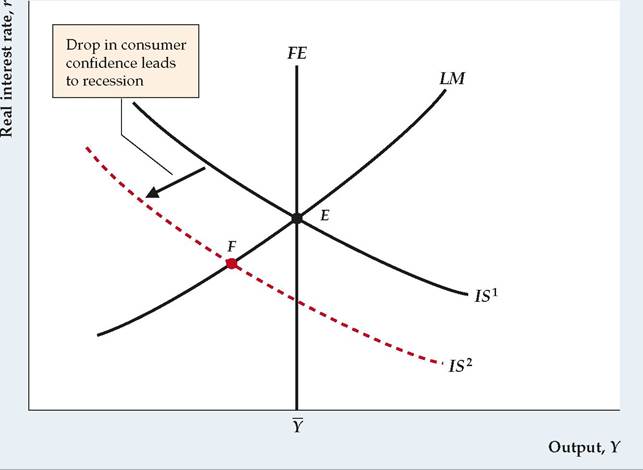
Figure 11.7 uses the Keynesian model to illustrate a recession caused by an aggregate demand shock. Suppose that consumers become pessimistic about the long-term future of the economy and thus reduce their current desired consumption; equivalently, they raise their current desired saving.
For any level of income, an increase in desired saving lowers the real interest rate that clears the goods market and thus shifts the IS curve down, from IS1 to IS2. The economy goes into recession at point F, and, as prices don't adjust immediately to restore full employment, it remains in recession for some period of time with output below its full-employment level. Because firms face below-normal levels of demand, they also cut employment.Note that a decline in investment spending (reflecting, for example, pessimism of business investors) or reduced government purchases would have similar recessionary effects as the decline in consumer spending analyzed in Fig. 11.7. Alternatively, a shift up and to the left of the LM curve (because of either increased money demand or reduced money supply) also could cause a recession in the Keynesian framework; in this case, high real interest rates caused by the "shortage" of money would cause the declines in consumer spending and investment. Thus Keynesians attribute recessions to "not enough demand" for goods, in contrast to classical economists who attribute recessions to "not enough supply."
FIGUREJ1.7
A recession arising from an aggregate demand shock
The figure illustrates how an adverse aggregate demand shock can cause a recession in the Keynesian model. The economy starts at general equilibrium at point E.
A decline in consumer confidence about the future of the economy reduces desired consumption and raises desired saving so that the IS curve shifts down, from IS1 to IS 2. The economy falls into recession at point F, with output below its fullemployment level, Y.
Like the real business cycle theory, the Keynesian theory of cycles can account for several of the business cycle facts: (1) In response to occasional aggregate demand shocks, the theory predicts recurrent fluctuations in output; (2) the theory correctly implies that employment will fluctuate in the same direction as output; and (3) because it predicts that shocks to the money supply will be nonneutral, the theory is consistent with the business cycle fact that money is procyclical and leading.
A business cycle fact that we previously emphasized (Chapter 8) is that spending on investment goods and other durable goods is strongly procyclical and volatile. This cyclical behavior of durable goods spending can be explained by the Keynesian theory if shocks to durable goods demand are themselves a main source of cycles. The demand for durable goods would be a source of cyclical fluctuations if, for example, investors frequently reassessed their expectations of the future MPK. Keynes himself thought that waves of investor optimism and pessimism, which he called "animal spirits," were a significant source of cyclical fluctuations. A rise in the demand for investment goods or consumer durables (at fixed levels of output and the real interest rate) is expansionary because it shifts the IS curve up and to the right. Investment will also be procyclical in the Keynesian model whenever cycles are caused by fluctuations in the LM curve; for example, an increase in the money supply, which shifts the LM curve down and to the right, both increases output and (by reducing the real interest rate) increases investment.
Another important business cycle fact that is consistent with the Keynesian theory is the observation that inflation tends to slow during or just after recessions (inflation is procyclical and lagging). In the Keynesian view, as Fig. 11.7 illustrates, during a recession, aggregate output demanded is less than the full-employment level of output. Thus when firms do adjust their prices, they will be likely to cut them to increase their sales. According to the Keynesian model, because demand pressure is low during recessions, inflation will tend to subside when the economy is weak.
Procyclical Labor Productivity and Labor Hoarding. Although the Keynesian model is consistent with many of the business cycle facts, one fact—that labor productivity is procyclical—presents problems for this approach. Recall that procyclical labor productivity is consistent with the real business cycle assumption that cycles are caused by productivity shocks—that recessions are times when productivity is unusually low and booms are times when productivity is unusually high.
Unlike the RBC economists, however, Keynesians assume that demand shocks rather than supply (productivity) shocks cause most cyclical fluctuations.Because supply shocks are shifts of the production function, the Keynesian assumption that supply shocks usually are unimportant is the same as saying that the production function is fairly stable over the business cycle. But if the production function is stable, increases in employment during booms should reduce average labor productivity because of the diminishing marginal productivity of labor. Thus the Keynesian model predicts that average labor productivity is countercyclical, contrary to the business cycle fact.
To explain the procyclical behavior of average labor productivity, Keynesians have modified their models to include labor hoarding. As discussed in Section 10.1, labor hoarding occurs if firms retain, or "hoard," labor in a recession rather than laying off or firing workers. The reason that firms might hoard labor during a recession is to avoid the costs of letting workers go and then having to rehire them or hire and train new workers when the recession ends. Thus hoarded labor may be used less intensively (for example, store clerks may wait on fewer customers in a day) or be assigned to activities such as painting, cleaning, maintaining equipment, and training. If labor is utilized less intensively during a recession, or workers spend time on activities such as maintenance that don't directly contribute to measured output, labor productivity may fall during a recession even though the production function is stable. Thus labor hoarding provides a way of explaining the procyclical behavior of average labor productivity without assuming that recessions and expansions are caused by productivity shocks.
Macroeconomic Stabilization
From the Keynesian explanation of why business cycles occur, we turn to the Keynesian view on how policymakers should respond to recessions and booms. Briefly, Keynesians—unlike classical economists—generally favor policy actions to "stabilize" the economy by eliminating large fluctuations in output and employment.
Keynesian support of more active policy measures follows from the theory's characterization of business cycle expansions and contractions as periods in which the economy is temporarily away from its general equilibrium (or not at the IS-LM-FE intersection). According to Keynesians, recessions are particularly undesirable because in a recession, employment may be far below the amount of labor that workers want to supply, which leads to hardships for the unemployed and to output that is "too low." Keynesians therefore argue that average economic well-being would be increased if governments tried to reduce cyclical fluctuations, especially recessions.The Keynesian analysis of monetary and fiscal policies suggests that these policies could be used to smooth the business cycle. To understand how, consider
FIGUREJ1.8
Stabilization policy in the Keynesian model From point E the economy is driven into a recession at point F by a drop in consumer confidence and spending, which shifts the IS curve down, from IS1 to IS 2. If the government took no action, in the long run price adjustment would shift the LM curve from LM1 to LM 2 and restore general equilibrium at point H (Scenario 1). Alternatively, the government could try to offset the recession through stabilization policy. For example, the Fed could increase the money supply, which would shift the LM curve directly from LM1 to LM 2, speeding the recovery in output (Scenario 2). Another possibility is a fiscal expansion, such as an increase in government purchases, which would shift the IS curve from IS 2 back to IS1, again restoring full employment at E (Scenario 3). Compared to a strategy of doing nothing, expansionary monetary or fiscal policy helps the economy recover more quickly but leads to a higher price level in the long run.
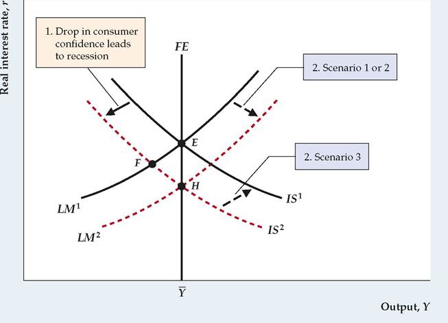
Figure 11.8. Suppose that the economy, initially in general equilibrium at point E, has been driven into recession at point F.
Various types of shocks could have caused this recession. In Fig. 11.7, for example, we considered a drop in consumer confidence about the future of the economy. A drop in confidence would reduce current desired consumption and increase current desired saving, thereby shifting the IS curve down from IS1 to IS2. This sort of change in consumer attitudes may have contributed to the 1990-1991 recession.How might policymakers respond to this recession? We consider three possible scenarios: (1) no change in monetary or fiscal policy, (2) an increase in the money supply, and (3) an increase in government purchases.
■ Scenario 1: No change in macroeconomic policy. One policy option is to do nothing. With no government intervention, the economy eventually will correct itself. At point F in Fig. 11.8,_aggregate output demanded is below the fullemployment level of output Y. Therefore, over time, prices will begin to fall, increasing the real money supply and shifting the LM curve down and to the right. In the long run, price declines shift the LM curve from LM1 to LM 2, restoring the economy to general equilibrium at point H. However, a disadvantage of this strategy is that, during the (possibly lengthy) price adjustment process, output and employment remain below their full-employment levels.
■ Scenario 2: An increase in the money supply. Instead of waiting for the economy to reach general equilibrium through price adjustment, the Fed could increase the money supply, which also would shift the LM curve from LM1 to LM 2 in Fig. 11.8. If prices adjust slowly, this expansionary policy would move the economy to general equilibrium at point H more quickly than would doing nothing.
■ Scenario 3: An increase in government purchases. An alternative policy of raising government purchases will shift the IS curve up and to the right, from IS2 to IS1. This policy also takes the economy to full employment, although at point E in Fig. 11.8 rather than at point H.
In all three scenarios, the economy eventually returns to full employment. However, the use of monetary or fiscal policy to achieve full employment leads to two important differences from the scenario in which no policy action is taken. First, if the government uses monetary or fiscal expansion to end the recession, the economy returns directly to full employment; if policy isn't changed, the economy remains in recession in the short run, returning to full employment only when prices have fully adjusted. Second, if there is no policy change (Scenario 1), in the long run the price level falls, which increases the real money supply, shifts the LM curve down and to the right, and restores full employment at point H. In contrast, when monetary or fiscal policy is used to restore full employment (Scenarios 2 and 3), the downward adjustment of the price level doesn't occur because expansionary policy directly returns aggregate demand to the full-employment level. (The real money supply, M/P, increases by the same amount in Scenario 1 and Scenario 2, but the increase in M/P is achieved by a reduction in P in Scenario 1 and by an increase in M, with unchanged P, in Scenario 2.) Thus according to the Keynesian analysis, using expansionary monetary or fiscal policy has the advantage of bringing the economy back to full employment more quickly but the disadvantage of leading to a higher price level than if no policy action is undertaken.
Usually, either monetary or fiscal policy can be used to bring the economy back to full employment. Does it matter which policy is used? Yes, there is at least one basic difference between the outcomes of the two policies: Monetary and fiscal policies affect the composition of spending (the amount of output that is devoted to consumption, the amount to investment, and so on) differently. In Fig. 11.8, although total output is the same at the alternative general equilibrium points E and H, at E (reached by an increase in government purchases) government purchases are higher than at H (reached by an increase in the money supply). Because government purchases are higher at E, the remaining components of spending— in a closed economy, consumption and investment—must be lower at E than at H. Relative to a monetary expansion, an increase in government purchases crowds out consumption and investment by raising the real interest rate, which is higher at E than at H. In addition, increased government purchases imply higher current or future tax burdens, which also reduces consumption relative to what it would be with monetary expansion.
Difficulties of Macroeconomic Stabilization. The use of monetary and fiscal policies to smooth or moderate the business cycle is called macroeconomic stabilization. Using macroeconomic policies to try to smooth the cycle is also sometimes called aggregate demand management because monetary and fiscal policies shift the aggregate demand curve. Macroeconomic stabilization was a popular concept in the heyday of Keynesian economics in the 1960s, and it still influences policy discussions. Unfortunately, even putting aside the debates between classicals and Keynesians about whether smoothing the business cycle is desirable, actual macroeconomic stabilization has been much less successful than the simple Keynesian theory suggests.
As discussed in connection with fiscal policy (Section 10.2), attempts to stabilize the economy run into some technical problems. First, because the ability to measure and analyze the economy is imperfect, gauging how far the economy is from full employment at any particular time is difficult. Second, the amount that output will increase in response to a monetary or fiscal expansion isn't known exactly. These uncertainties make assessing how much of a monetary or fiscal change is needed to restore full employment difficult. Finally, even knowing the size of the policy change needed still wouldn't provide enough information. Because macroeconomic policies take time to implement (the implementation lag discussed in Chapter 10) and more time to affect the economy (the impact lag discussed in Chapter 10), their optimal use requires knowledge of where the economy will be six months or a year from now. But such knowledge is, at best, very imprecise.
Because of these problems, aggregate demand management has been likened to trying to hit a moving target in a heavy fog. These problems haven't persuaded most Keynesians to abandon stabilization policy; however, many Keynesians agree that policymakers should concentrate on fighting major recessions and not try to fine-tune the economy by smoothing every bump and wiggle in output and employment.
Supply Shocks in the Keynesian Model
Until the 1970s, the Keynesian business cycle theory focused almost exclusively on aggregate demand shocks as the source of business cycle fluctuations. Because aggregate demand shocks lead to procyclical movements in inflation, however, the Keynesian theory failed to account for the stagflation—high inflation together with a recession—that hit the U.S. economy during the 1973-1975 recession, which was induced by a quadrupling of oil prices in 1973.
This experience led to much criticism of the traditional theory by both economists and policymakers, so Keynesians recast the theory to allow for both supply and demand shocks. Although Keynesians wouldn't go so far as to agree with RBC economists that supply (productivity) shocks are a factor in most recessions, they now concede that there have been occasional episodes—the oil price shocks of the 1970s being the leading examples—in which supply shocks have played a primary role in an economic downturn. (See "In Touch with Data and Research: DSGE Models and the Classical-Keynesian Debate," for further discussion of agreement and disagreement between Keynesians and classicals.)
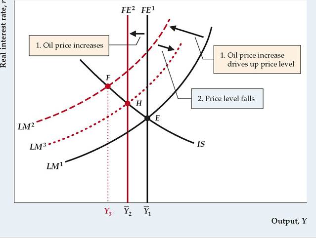
Figure 11.9 shows a Keynesian analysis of the effects of a sharp temporary increase in the price of oil (a similar analysis would apply to other supply shocks, such as a drought). As we showed in Chapter 3, if firms respond to an increase in the price of oil by using less energy, the amount of output that can be produced with the same amount of capital and labor falls. Thus the increase in the price of oil is an adverse supply shock, which reduces the full-employment level of output and shifts the FE line to the left, from FE1 to FE2. After complete wage and price adjustment, which occurs virtually immediately in the basic classical model but only in the long run in the Keynesian model, output falls to its new full-employment level, Y2. Thus in the long run (after full wage and price adjustment), the Keynesian analysis and the classical analysis of a supply shock are the same.
However, the Keynesian analysis of the short-run effects of an oil price shock is slightly different from the classical analysis. To understand the short-term effects of the oil price shock in the Keynesian model, first think about the effects of the increase in the oil price on the general price level. Recall that firms facing menu
FIGUREJ1.9
An oil price shock in the Keynesian model An increase in the price of oil is an adverse supply shock that reduces full-employment output from Y1 to Y2 and thus shifts the FE line to the left. In addition, the increase in the price of oil increases prices in sectors that depend heavily on oil, whereas prices in other sectors remain fixed in the short run. Thus the average price level rises, which reduces the real money supply, M∕P, and shifts the LM curve up and to the left, from LM1 to LM2. In the short run, the economy moves to point F, with output falling below the new, lower value of fullemployment output and the real interest rate increasing. Because the aggregate quantity of goods demanded at F is less than the fullemployment level of output, Y2, in the long run the price level falls, partially offsetting the initial increase in prices. The drop in the price level causes the LM curve to shift down and to the right, from LM2 to LM 3, moving the economy to full-employment equilibrium at point H.
costs will not change their prices if the "right" prices are only a little different from the preset prices. However, if the right prices are substantially different from the preset prices, so that firms would lose considerable profits by maintaining the preset prices, they will change their prices. In the case of a large increase in the price of oil, firms whose costs are strongly affected by the price of oil—including gas stations, suppliers of home heating oil, and airlines, for example—find that the right prices for their products are substantially higher than the preset prices. These oil-dependent firms increase their prices quickly, whereas firms in other sectors maintain their preset prices in the short run. Thus there is price stickiness in the sense that not all prices adjust to their equilibrium values, and yet the average price level rises in the short run.
Because a sharp increase in the price of oil raises the price level, P, in the short run, it also reduces the real money supply, M∕P. A decline in the real money supply shifts the LM curve up and to the left, from LM1 to LM2 in Fig. 11.9. As drawn, the intersection of the LM curve and the IS curve is located to the left of the new FE line, although this outcome isn't logically necessary. The short-run equilibrium is at point F, where LM2 intersects the IS curve. Because F is to the left of the FE line, the economy is in a recession at F, with output (at Y3) below the new value of full-employment output, Y2. In the short run, the economy experiences stagflation, with both a drop in output and a burst of inflation. Note that, according to this analysis, the short-run decline in output has two components: (1) the drop in full-employment output from Y1 to Y2 and (2) the drop in output below the new full-employment level arising from the shift up and to the left of the LM curve (the difference between Y2 and Y3).
Supply shocks of the type analyzed in Fig. 11.9 pose tremendous difficulties for Keynesian stabilization policies. First, monetary or fiscal policy can do little
In Touch with Data and Research
DSGE Models and the Classical-Keynesian Debate
In Chapters 10 and 11, we have compared and contrasted the classical and Keynesian approaches to analyzing the business cycle and to determining stabilization policy. For many years, classical and Keynesian economists pursued research on business cycles and stabilization policy using very different types of models, and they argued about the data using very different empirical methods. As a result, communication between the two groups was difficult. (See Table 11.1 for a comparison of the classical view and the Keynesian view.)
However, in the past 20 years, some classical economists have been incorporating Keynesian ideas into their models, and some Keynesian economists have been incorporating classical ideas into their models. Many young economists coming from top Ph.D. programs have been well trained in dynamic, stochastic, general equilibrium (DSGE) models, which we discussed briefly in Chapter 10. Roughly speaking, those models use techniques that were developed by classical RBC economists in the 1980s and 1990s, and many Keynesian economists have adopted classical methods of analysis.20 But many of the models, even those used by classical economists, incorporate Keynesian features, especially sticky prices (but not usually efficiency wages) and imperfect competition among firms. As a result, classical and Keynesian economists are now speaking the same language and can communicate with each other more clearly, and research on macroeconomic ideas is advancing more smoothly. Their research is increasingly being used to influence policymakers, as DSGE models incorporating sticky prices and financial factors are increasingly used by central banks for applied policy analysis.
20See, for example, Michael Woodford, Interest and Prices: Foundations of a Theory of Monetary Policy (Princeton, NJ: Princeton University Press, 2003).
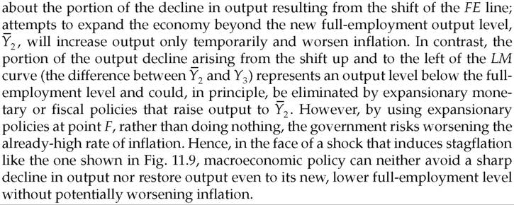
TABLE 11.1
Comparing the Keynesian View with the Classical View
| Category | Classical View | Keynesian View |
| How fast does the price level adjust to restore general equilibrium? | Quickly | Slowly |
| What type of model is appropriate? | A model with microeconomic foundations | An aggregate model |
| Are supply shocks important? | They are the most important shocks | Aggregate demand shocks are more important |
| What is the role for government intervention in the economy? | Government intervention is usually unwarranted | Government intervention is vital |
| Do inflation and inflation expectations matter? | Yes, they matter | No, they do not matter much |
| What type of model is best? | A dynamic model | A static model is fine |
| What model of unemployment is appropriate? | A matching model of unemployment | A disequilibrium model of unemployment |
| Where is the equilibrium in the labor market? | Where the labor supply curve intersects the labor demand curve | Where the efficiency wage hits the labor demand curve |
| Does a shift in labor supply affect the FE line? | Yes | No |