References and Literature

The early development literature contains many important works documenting the ma­jor structural changes taking place in the process of development. Kuznets (1957, 1973) and Chenery (1960) provide some of the best overviews of the broad evidence and the litera­ture, though similar issues were discussed by even earlier development economists such as Rosenstein-Rodan (1943), Nurske (1953), and Rostow (1960).

The model of non-balanced growth based on Engel’s law presented in Section 20.1 is based on Kongsamut, Rebelo and Xie (2001). Previous work that have analyzed similar models in­clude Murphy, Shleifer and Vishny (1989), Echevarria (1997), Laitner (2000). More recent work building on Kongsamut, Rebelo and Xie (2001) includes Caselli and Coleman (2001) and Gollin, Parente and Rogerson (2002). Many of these models are considerably richer than the Kongsamut, Rebelo and Xie approach. For example, Murphy, Shleifer and Vishny (1989) incorporate monopolistic competition and analyzes the implications of income inequality for the demand for different types of goods. Echevarria (1997) and Laitner (2000) show how the initial phase of transitioning from agriculture to manufacturing will be associated with aggre­gate non-balanced growth. The distinguishing feature of these models is that land is also a factor of production and is more important for agriculture than for manufacturing. Exercise 20.8 provides an example of such a model. The recent literature also places greater emphasis 843

on sources of agricultural productivity and emphasizes that differences in agricultural pro­ductivity across countries are often as large as or even larger than productivity differences in other sectors. Gollin, Parente and Rogerson (2002) is one of the first papers in this vein.

The works mentioned in the previous paragraph, like the model I presented in Section

20.1, appeal to Engel’s law and model the resulting non-homothetic preferences by positing Stone-Geary preferences as in equation (20.3). A more flexible and richer approach is to allow for “hierarchies of needs” in consumption, whereby households consume different goods in a particular sequence (e.g., food need to be consumed before textiles, and textile need to be consumed before electronics, etc.). This approach is used in Stokey (1988), Matsuyama (2002), Foellmi and Zweimuller (2002), and Buera and Kaboski (2006) to generate richer models of structural change. Space restrictions precluded me from presenting these hierarchy of needs models, even though they are both insightful and elegant alternatives to the standard approach of using Stone-Geary preferences.

Section 20.2 builds on Acemoglu and Guerrieri (2006). The precursor to this work is Baumol (1967), which emphasized the importance of differential productivity growth on non­balanced growth. However, Baumol did not derive a pattern of non-balanced growth including reallocation of capital and labor across sectors, and assumed differential rates of productivity growth to be exogenous. Ngai and Pissarides (2006) and Zuleta and Young (2006) provide modern versions of Baumol’s hypothesis. Instead, the approach in Section 20.2 emphasizes how the combination of different capital intensities and capital deepening in the aggregate can endogenously lead to this pattern.

The model in Section 20.3 is based on Matsuyama (1992) and is also closely related to the model I presented in Section 19.7 in Chapter 19. Excellent account of the role of agriculture in industrialization, especially in the British context, are provided in Mokyr (1993) and Overton (2001).

20.5. Exercises

Exercise 20.1. (1) Show that the consumption aggregator in (20.3) leads to Engel’s

law.

(2) Suggest alternative consumption aggregators that will generate similar patterns.

Exercise 20.3. (1) Set up the optimal control problem for a representative household

in the model of Section 20.1.

(2) From the Euler equations and the transversality condition, verify part 1 of Proposi­tion 20.2.

(3) Use equations (20.10)-(20.11) to derive parts 2 and 3 of the proposition.

Exercise 20.4. (1) Prove Proposition 20.3.

844

(2) Show that even though a balanced growth path does not exist, an equilibrium path always exists.

Exercise 20.5. (1) Prove Proposition 20.4. In particular, show that if (20.21) is not

satisfied, a CGP cannot exist, and that this condition is sufficient for a CGP to exist.

(2) Characterize the CGP effective capital-labor ratio, k*.

Exercise 20.6. In the model of Section 20.1, show that as long as condition (20.21) is satisfied when the economy starts with an effective capital-labor ratio K (0) / (X (0) L (0)) different from k*, the CGP is globally stable and the effective capital-labor ratio will monotonically converge to k* as t → ∞.

Exercise 20.7. * Consider a generalization of the model of Section 20.1, where the sectoral production functions are given by the following Cobb-Douglas forms

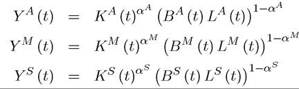
and assume that BA (t), B^m (t) and B^s (t) grow respectively at the rates g^A, g^M and g^s.

(1) Derive the equivalent of Propositions 20.1 and 20.2.

(2) Show that as long as preferences are given by (20.3) and balanced growth is impossible.

(3) Show that there exists a generalization of condition (20.21) such that this model will have a CGP as defined in Section 20.1. [Hint: the generalization includes two separate conditions that depend on technology growth rates as well as preference parameters].

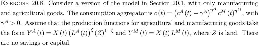
(1) Characterize the competitive equilibrium in this economy.

(2) Show that this economy also exhibits structural change; in particular, show that the share of manufacturing sector grows over time.

(3) What happens to land rents along the equilibrium path?

Exercise 20.9. * In the model of Section 20.1, suppose that condition (20.21) is not satisfied. Assume that the production function F is Cobb-Douglas. Characterize the asymptotic growth path of the economy (i.e., the growth path of the economy as t → ∞).

(2) State and prove the equivalent of Proposition 20.11, when the converse of condition (20.64) holds.

Exercise 20.15. Show that in the allocation in Proposition 20.11 the asymptotic interest rate is constant and derive a closed-form expression for this interest rate.

Exercise 20.16. * In this exercise, you are first asked to provide an alternative proof of

Proposition 20.11 and then characterize the local transitional dynamics in the neighborhood of the constant growth path.

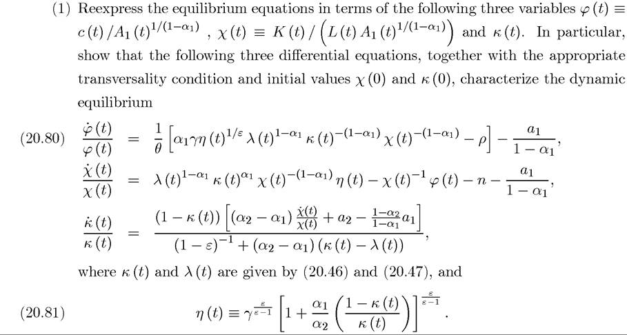
[Hint: use the Euler equation of the representative consumer and the resource con­straint of the economy, rearrange these to express the laws of motion of φ (t) and

χ (t) in terms of κ (t), λ (t) and η (t) as defined in (20.81), and then differentiate (20.46).]

(2) State the appropriate transversality condition.

(3) Show that if an allocation satisfies the three differential equations in (20.80) and the appropriate transversality condition, then it corresponds to an equilibrium path.

(4) Show that in a CGP equilibrium φ (t) must be constant. Using this, show that the CGP requires that κ (t) → 1 and that χ (t) be constant. From these observations, derive an alternative proof of Proposition 20.11.

(5) Now linearize these three equations around the CGP of Proposition 20.11 and show that the linearized system has two negative and one positive eigenvalues and using this fact conclude that the constant growth path is locally stable.

EXERCISE 20.17. Consider a model that combines the supply-side and the demand side fea­tures discussed in Sections 20.1 and 20.2. In particular, suppose that the consumption aggre­gator is given by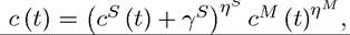where c^s consumption of services and c^M

denotes the consumption of manufacturing goods. Assume that the economy is closed and both services and manufacturing are produced by Cobb-Douglas technologies with the same Hicks-neutral rate of exogenous technological progress, but manufacturing is more capital­intensive. Characterize the equilibrium of this economy. Show that the relative price and the employment share of services will be increasing over time. Is it possible for the total consumption of manufacturing goods to increase faster than those of services?

Exercise 20.18. Consider the model of Section 20.3.

(1) Show that aggregate food (agricultural) consumption and production stay constant at

(2) Show that this is increasing in BA and provide the intuition for this result.

(3) Show that expenditure on agricultural goods increases at the same rate as aggregate output. [Hint: first characterize how p (t) changes along the equilibrium path].

Exercise 20.19. * Consider the model of Section 20.3 and suppose that the production function for the manufacturing sector is given by

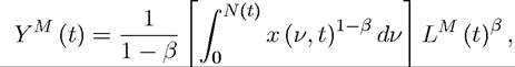
which is similar to the production functions in Part 4 of the book, with N (t) denoting the range of machines (intermediates) and x (ν, t) corresponding to the amount of machine of

847

type ν used by the manufacturing sector.

15.7. Characterize the equilibrium of this economy and show that the qualitative features are the same as the model in the text.

Exercise 20.20. Consider an open economy version of the model of Section 20.3. In par­ticular, suppose that the economy trades with the rest of the world taking product prices as given. The rest of the world is characterized by the same technology, except that it has an initial level of productivity in the manufacturing sector equal to X^f (0) and an agricultural productivity given by A^f. Suppose that there are no spillovers in learning-by-doing, so that equation (20.74) applies to the “home” economy and the law of motion of manufacturing productivity in the rest of the world is given by X^f (t) = δY^m,f (t), where Y^m,f (t) is total foreign manufacturing production at time t.

(1) Show that comparative advantage in this economy is determined by the comparison of X (0) /B^a versus X^f (0) /A^f. Interpret this.

(2) Supposethat X (0) /B^a < X^f (0) /B^f, so that the home economy has a comparative advantage in agricultural production. Show that the initial share of employment in manufacturing in the home economy, n* (0), must satisfy

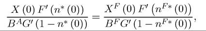
whereis the share of manufacturing employment in the rest of the world. Show that n* (0) given by this equation is strictly less than n* as given by (20.79).

(3) What happens to manufacturing employment in the home economy starting as in part 2 of this exercise? [Hint: derive an equivalent of the equation in part 2 for any t, differentiate this with respect to time and then use the laws of motion of X and X ^f ].

(4) Explain why agricultural productivity, which was conducive to faster industrializa­tion in the closed economy, may lead to delayed industrialization or to deindustrial­ization in the open economy.

(5) Consider an economy specializing in agriculture as in the earlier parts of this exercise. Is welfare at time t = 0 necessarily lower when this economy is open to trade than when it is closed to trade? Relate your answer to the analysis in Section 19.7 of Chapter 19.