Risk, Diversification and Growth

In this section, I present a stochastic model of long-run growth based on Acemoglu and Zilibotti (1997). This model is useful for two distinct purposes. First, because it is simpler than the baseline neoclassical growth model under uncertainty, it will provide a complete characterization of the stochastic dynamics of growth and show how simple ideas from the theory of Markov processes can be used in the context of the study of economic growth.

“The advance occurred very slowly over a long period and was broken by sharp recessions. The right road was reached and thereafter never abandoned, only during the eighteenth century, and then only by a few privileged countries.

In the model I will present here, these patterns arise endogenously because the extent to which the economy can diversify risks by investing in imperfectly correlated activities is limited by the amount of capital it possesses. As the amount of capital increases, the economy achieves better diversification and faces fewer risks. The resulting equilibrium process thus generates greater variability and risk at the early stages of development and these risks are significantly reduced after the economy manages to “take off” into sustained growth. Moreover, the desire of individual households to avoid risk makes them invest in lower return less risky activities during the early stages of development, thus the growth rate of the economy is also endogenously limited during this pre-takeoff stage. In addition, in this economic development goes hand-in-hand with financial development as greater availability of capital enables better risk sharing through asset markets. Finally, because the model is one 670

of endogenously incomplete markets, it also enables us to show that price-taking behavior by itself is not sufficient to guarantee Pareto optimality, and the form of inefficiency of the equilibrium in this economy will be interesting both on substantive and methodological grounds.

17.6.1. The Environment. We consider an overlapping generations economy. Each generation lives for two periods. There is no population growth and the size of each generation is normalized to 1. The production sector consists of two sectors. The first sector produces final goods with the Cobb-Douglas production function

where as usual L (t) is total labor and K (t) is the total capital stock available at time t. Capital depreciates fully after use (i.e., δ = 1 in terms of our previous notation).

The second sector transforms savings at time t — 1 into capital to be used for production at time t. This sector consists of a continuum [0,1] of intermediates, and stochastic elements only affect this sector. In particular, let us represent possible states of nature also with the unit interval and assume that intermediate sector j ∈ [0,1] pays a positive return only in state j and nothing in any other state. This formulation implies that investing in a sector is equivalent to buying a Basic Arrow Security that only pays in one state of nature. Since there is a continuum of sectors, the probability that a single sector will have positive payoff is 0, but if an individual invests in some subset J of [0,1], then there will be positive returns with probability equal to the (Lebesgue) measure on the set J. Thus each intermediate sector is a risky activity but an individual (and in particular, the representative household in the economy) can diversify risks by investing in multiple sectors. In particular, if one were to invest in all of the sectors, then one would receive positive returns with probability 1. What makes the economic interactions in this model non-trivial is that investing in all sectors will not be possible at every date because of potential nonconvexities. More specifically, we assume that each sector has a minimum size requirement, denoted by M (j) and positive returns will be realized only if aggregate investment in that sector exceeds M (j).

In light of this description, let I (j, t) be the aggregate investment in intermediate sector j at time t. We assume that this investment will generate date t +1 capital equal to QI (j, t) if state j is realized and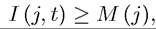and nothing otherwise. Thus aggregate investment in

the intermediate sector exceeding the minimum size requirement is necessary for any positive returns.

In addition to the risky intermediate sectors, we assume that there is also a safe interme­diate sector which transforms one unit of savings at date t into q units of date t + 1 capital.

671

so that the safe option is also less productive.

The requirement that I (j,t) ≥ M (j) combined with the fact that the amount of capital obtained from savings I (j, t) in state j is equal to QI (j, t) implies that all intermediate sectors have linear technologies, but only after the minimum size requirement, M (j), is met. For any I (j, t) < M (j), the output is equal to 0. In order to simplify the exposition and the computations, let us adopt a simple distribution of minimum size requirements by intermediate sector:

This equation implies that intermediate sectorshave no minimum size requirement, so aggregate investments of any size can be made in the sectors. For the remaining sectors, the minimum size requirement increases linearly. Figure 17.2 shows the minimum size require­ments with the thick line. This figure will be used to illustrate the determination of the set of open sectors once the equilibrium investments are specified.

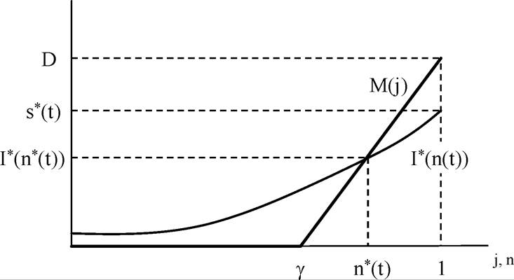
Figure 17.2. Minimum size requirements, M (j), of different sectors and demand for assets, I* (n).

It is worth noting that there are three important features introduced so far.

(1) Risky investments have a higher expected return than the safe investment, which is captured by the assumption that Q > q.

(2) The output of the risky investments (of the intermediate sectors) are imperfectly correlated so that there is safety in numbers.

(3) The mathematical formulation here implies a simple relationship between invest­ments and returns. As already hinted above, if an individual holds a portfolio consisting of an equi-proportional investment I in all sectors, and the

(Lebesgue) measure of the set J is p, then the portfolio pays the return QI with probability p, and nothing with probability 1 — p.

The first two features imply that if the aggregate production set of this economy had been convex, for example because D = 0, all agents would invest an equal amount in all inter­mediate sectors and manage to diversify all risks without sacrificing any of the high returns. However, in the presence of nonconvexities, as captured by the minimum size requirements, there is a tradeoff between insurance and high productivity.

Let us next turn to the preferences of households. Recall that each generation has size normalized to 1. Consider a household from a generation born at time t. The preferences of this household are given by

where ci (t) is the consumption of final goods in the first period of this household’s life (which is at time t) and c2 refers to consumption in the second period of this household. E_t refers to the expectations operator, because second period consumption is risky. This is spelled out on the right-hand side of (17.37), with c2 (j,t + 1) denoting consumption in state j at time t. The integral replaces the expectation using the fact that all states are equally likely. As in the canonical overlapping generations model, each household has 1 unit of labor when young and no labor endowment when old. Thus the total supply of labor in the economy is 1. Moreover, in the second period of their lives, each individual consumes the return from their savings. For future reference, the set of young households at time t is denoted by H_t and Figure 17.3 depicts the life cycle and the various decisions of a typical household, emphasizing that uncertainty affects the return on their savings and thus the amount of capital they will have in the second period of their lives.

The aggregate capital stock depends on the realization of the state of nature, which determines how much of the investments in different intermediate sectors at time t is turned into capital.

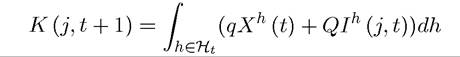
where I^h (j, t) is the amount of savings invested by (young) agent h ∈ H_t in sector j at time t, and X^h (t) is the amount invested in the safe intermediate sector.

673

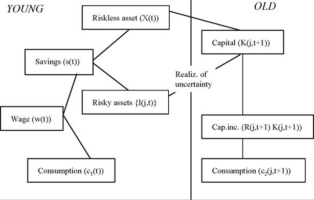
Figure 17.3. Life cycle of a typical household.

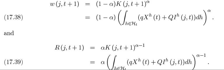
Since the capital stock is potentially random, so will be output and factor prices. In particular, both labor and capital are assumed to be traded in competitive markets, so the equilibrium factor prices will be given by their marginal products. Since the total capital stock in state j at time t + 1 is K (j,t + 1) and the total supply of labor is equal to 1, these prices are given by

To complete the description of the environment, we also specify the market structure of the intermediate sector. We assume that households make investments in different intermediate sectors through financial intermediaries. There is free entry into financial intermediation (either by a large number of firms or by the households themselves). Any intermediary can form costlessly and mediate funds for a particular sector, that is, it can collect funds, invest them in a particular intermediate sector and give corresponding Basic Arrow Securities to its investors. The important requirement is that, to be able to invest, any financial intermediary should raise enough funds to cover the minimum size requirement. For now, we assume 674

that each financial intermediary can operate only a single sector.^[39] Thus we are ruling out the formation of a grand financial intermediary managing all investments. We return to this issue in subsection 17.6.5. We denote the price charged for a security associated with intermediate sector j at time t by P (j, t). Although the decentralized equilibrium in this economy will be defined and analyzed in the next section, we can already make a few useful observations about the prices for the securities, the P (j, t)s. Clearly P (j, t) < 1 is not possible, since one unit of the security requires one unit of the final good, so P (j, t) < 1 would lose money. What about P (j, t) > 1? This is also ruled out by free entry. Imagine that a particular intermediary offers security j at some price P (j, t) > 1 and raises enough funds so that the total investment in this intermediate sector I (j, t) is greater than the minimum size requirement M (j). But in that case, some other intermediary can also enter, offer a lower price for the security, and attract all the funds that were otherwise received by the first intermediary. This argument shows that P (j, t) > 1 is not possible either, so that equilibrium behavior will force P (j, t) = 1 for all securities that are being supplied. However, we will see that securities for not all intermediate sectors will be supplied in equilibrium.

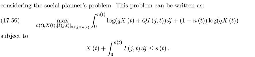
17.6.2. Equilibrium. We now characterize the equilibrium of the economy described in the previous subsection. Recall the two observations from the previous paragraph. First, not all intermediate sectors will be open at each date, meaning that there will be securities for only a subset of the intermediate sectors at any date. Let the set of intermediate sectors that are open at date t be denoted by J (t). Second, by the argument at the end of the previous subsection, for any j ∈ J (t) free entry implies that P (j,t) = 1. These two observations enable us to write the problem of a representative householdtaking prices and the set of available securities at time t as given. This problem takes the following form:

subject to: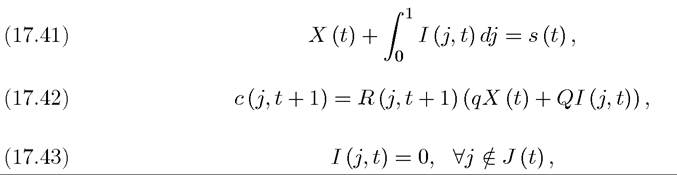

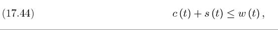
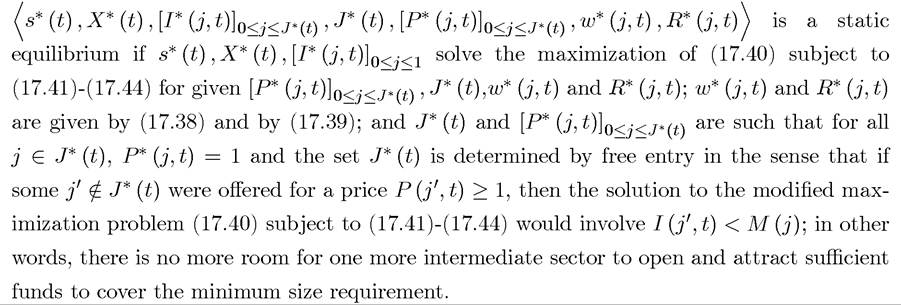
where I have suppressed the superscript h to simplify the notation. Here equation (17.40) is the expected utility (objective function) of the representative household. Equations (17.41)­(17.44) are the constraints on this maximization problem. The first one, (17.41), requires that the investment in the safe sector and the sum of the investments in all other securities are equal to the total savings of the individual, s (t). Equation (17.42) expresses consumption of the individual in state j at time t +1. Two features are worth noting. First, recall households supply labor only when young and consume capital income when old. This implies that second period consumption for the household is equal to its capital holdings times the rate of return to capital, R (j,t + 1) given by (17.39). This rate of return is conditioned on the state j (at time t + 1) since the amount of capital and thus the marginal product of capital will differ across states. Second, the amount of capital available to the household is equal to what it receives from the safe investment, qX (t), plus the return from the Basic Arrow Security for state j, QI (j,t). Equation (17.43) encapsulates a major constraint on household behavior: it emphasizes that the household cannot invest in any security that is not being supplied in the market. In particular, recall that I (j, t) ≥ M (t) is necessary for an intermediate sector to be open and this may not be possible for all sectors in [0,1], so some subset of the sectors in [0,1] may not be open and thus there will not be securities for the sectors that are not traded in equilibrium. Naturally, the household cannot invest in these non-traded securities and the constraint (17.43) ensures this. Finally, (17.44) requires the sum of consumption and savings to be less than or equal to the income of the individual, which only consists of his wage income, given by (17.38).

We are now in a position to define an equilibrium. We do this in two steps. A static equilibrium is an equilibrium for time t, taking the amount of capital available at time t, K (t), and thus the wage w (t) as given. A time t tuple

A dynamic equilibrium is a sequence of static equilibria linked to each other through (17.38) given the realization of the state j (t) at each t = 1, 2,...

676

Because preferences in (17.40) are logarithmic, the saving rate of all households will be constant as in the canonical overlapping generations model. Consequently, we obtain the following saving rule regardless of the risk-return tradeoff:

Given this result, a household’s optimization problem can be broken into two parts: first, the amount of savings is determined, and then an optimal portfolio is chosen. This decomposition of the optimization problem is particularly useful because of two observations (with proofs left as exercises):

(1) For any j,j⁰ ∈ J (t), we have that I * (j, t) = I * (j⁰,t). Intuitively, since each individ­ual is facing the same price for all of the traded symmetric Basic Arrow Securities, he would want to purchase an equal amount of each and thus achieving a balanced portfolio (see Exercise 17.23).

(2) The set of open projects at time t will take the form J* (t) = [0,n* (t)] for some n (t) ∈ [0,1]. Intuitively, when only a subset of projects can be opened in equilibrium, intermediate sectors with small minimum size requirements will be opened before those with greater minimum size requirements. Consequently, if an intermediate sector j* is open, all sectors j ≤ j* must also be open (see Exercise 17.24).

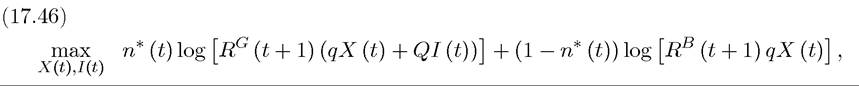
The previous two observations also imply that we can divide the states of nature at time t into two sets: states in [0,n (t)] that are “good” in the sense that the society is lucky and its risky investments have delivered positive returns, and states in (n (t), 1] that are “bad” in the sense that the society is unlucky and its risky investments have zero returns. Clearly, the rate of return to capital (and the wage rate) will take different values in these two sets of states. We denote the rate of return to capital when a good state is realized by R^g (t + 1) and when a bad state is realized by R^b (t + 1) —these returns are dated t + 1, because they are paid out at time t + 1. In light of this structure, the maximization problem of a representative household can be written in the much simpler form:

subject to:

677

is the marginal product of capital in the “bad” state, when the realized state is j > n* (t) and no risky investment pays off, and

applies in the “good state”, i.e. when the realized state is

Straightforward maximization of (17.46) subject to (17.47) yields the unique solution to the household’s problem as:

and

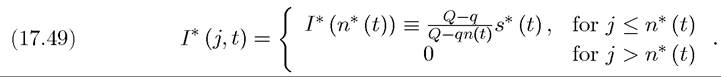
Notably, equation (17.49) implies that the demand for each asset (or investment in each intermediate sector) grows as the measure of open sectors increases, i.e., I* (n) is strictly increasing in n. This is because when more securities are available, the risk-diversification opportunities improve and consumers become willing to reduce their investments in the safe asset and increase their investments in risky projects. This represents an important economic force. What holds back investment in the higher productivity sectors in this economy is the fact that they are riskier than the safe sector. But since there is “safety in numbers,” that is, a first-order benefit from diversification, when there are financial assets traded on more sectors, each household is willing to invest more in risky assets in total. This complementarity between the set of traded assets and investments will play an important role in the dynamics of economic development below.

Equations (17.45), (17.48) and (17.49) completely characterize the utility-maximizing behavior of the representative household given the set of intermediate sectors that are active. To completely characterize the equilibrium, we need to find the set of sectors that are active. We know that this is equivalent to finding a threshold sector n* (t) such that all can meet their minimum size requirements while no additional sector can enter and raise enough funds to meet its minimum size requirements. Diagrammatically, this can be done by plotting the level of investment for each sector in a balanced portfolio, I * (n* (t)) given by (17.49), together with the minimum size requirement, M (j) given by (17.36). The first curve can be loosely interpreted as the “demand for assets” in the financial market and the curve for (17.36) can be thought of as corresponding to the “supply of assets”. The two curves and their intersection is plotted in Figure 17.2. The figure shows a unique intersection between the two curves. However, because both curves are upward-sloping, more than one intersection is possible in general. It can be verified that the condition Q ≥ (2 — γ) q is sufficient to ensure a unique intersection (see Exercise 17.25). If this condition is violated, there might be multiple solutions, corresponding to multiple equilibria. These equilibria would involve different number of active sectors. When there are only a few active sectors, households invest a large fraction of their resources in the safe asset, and in equilibrium only a few risky sectors can be operated. In contrast, when there is a significant number of active risky sectors, each household invests a large fraction of its resources in risky assets. This enables more sectors to be open and creates better risk diversification for all households. When such multiple equilibria exist, the equilibrium with more active sectors gives higher ex ante utility to all households. While interesting for illustrating the forces at work, one would expect that financial intermediaries might be successful in avoiding this type of coordination failures. Motivated by this reasoning, let us focus on on the part of the parameter space where Q ≥ (2 — 7) q. In that case, the static equilibrium is uniquely defined and the following proposition summarizes this equilibrium.

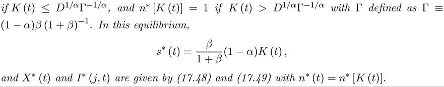
Proposition 17.8. Suppose that Q ≥ (2 — 7) q and that K (t) is given. Then there exists a unique time t equilibrium in which all sectors j ≤ n* (t) = n* [K (t)] are open and those j > n* [K (t)] are shut, where

Proof. See Exercise 17.26.

?

An important feature is that the equilibrium threshold sector n^* [K] is increasing in K. When there is more capital, the economy is able to open more intermediate sectors. This again contributes to the complementarity in the behavior mentioned above, since equation (17.49), in turn, implies that when there are more open sectors, investment in each sector will increase.

17.6.3. Equilibrium Dynamics. We next turn to the characterization of equilibrium dynamics. Given the static equilibrium in Proposition 17.8, it is straightforward to charac­terize the full stochastic equilibrium process. The law of motion for the capital stock, K (t), will be given by a simple Markov process. Recall that investments in risky sectors will be successful with probability n* [K (t)] when the capital stock is K (t), and it will be unsuccess­ful with the complementary probabilityThis implies the following stochastic

law of motion for the capital stock:

where n* [K (t)] is given by equation (17.50) and recall that Γ ? (1 — α)β (1 + β)^-1. Notice that the first line of (17.51) is always less than the second line, which reflects the fact that the second line refers to the case in which the investments in the intermediate sectors have been successful.

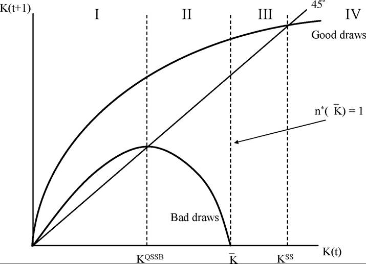
Figure 17.4. The stochastic correspondence of the capital stock.

Equation (17.51) is a particularly simple Markov process, since given K (t), K (t + 1) can only take two values. However, it is a Markov process not a Markov chain, since for different values of K (t), the possible values of K (t + 1) belong to the entire R₊. A diagrammatic analysis of this Markov process is particularly illuminating. Consider Figure 17.4, which plots the stochastic correspondence of the Markov process in (17.51) and is thus similar to Figure 17.1 in the previous section. The main difference is that in Figure 17.1, any value between the two curves for z_mi_n and z_max were possible. In contrast, here, only values exactly on the two curves plotted in the figure are possible. The first curve corresponds to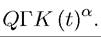This is the

value of the capital stock that would result if households followed their equilibrium investment strategies given in (17.48) and (17.49), and at each date, the economy turned out to be lucky, 680

so that their investments always had positive return. The second, inverse U-shaped curve correspondand thus applies if the economy

is unlucky at each date. Both curves start above the 45⁰ line near zero for the same reason as that given for the similar pattern in Figure 17.1 (i.e., because the aggregate production function (17.34) satisfies the Inada conditions). The economy will be on the upper curve with probability n* [K (t)] and on the lower curve with probability 1 — n* [K (t)]. This implies that not only do the probabilities of success and failure change with the aggregate capital stock but so does average productivity. To quantify this variation in average productivity, let us define expected total factor productivity (TFP) conditional on the proportion of intermediate sectors that are open:

Straightforward differentiation establishes thatis strictly increasing in

n* [K (t)]. This implies that as the economy develops and manages to open more inter­mediate sectors, its productivity will endogenously increase. Since n^* [K] is increasing in K, this implies that average productivity is increasing in the capital stock of the economy. We record this as a proposition for future reference:

Proposition 17.9. The expected total factor productivity of the economyis

increasing in n* and thus increasing in K.

Inspection of Figure 17.4 also suggests that the following two levels of capital stock are special and useful in the analysis.

(i) : K^qssb refers to the “quasi steady state” of an economy which always has unlucky draws. An economy would converge towards this quasi steady state if it follows the optimal investments characterized above but the sectors chosen by the households never have positive pay-off due to bad luck.

(ii) : K^qssg refers to the “quasi steady state” of an economy which always receives good news, meaning that it is always on the upper curve in Figure 17.4.

These two capital stock levels are plotted in the figure and are also easy to compute as:

The form ofis particularly noteworthy, since it refers to the case in which the economy never faces any risk and thus acts very much like a standard neoclassical growth model. In particular, if, in equilibrium,in fact becomes a

proper steady state and the economy would stay at this level of capital stock once it reaches 681

it. This is because once the economy accumulates sufficient capital to open all intermediate sectors, it would eliminate all risk and would always be on the upper curve in Figure 17.4.

Equations (17.50) and (17.53) show that the condition for this good steady state to exist, i.e., foris that the saving level corresponding to K^qssg be sufficient to

ensure a balanced portfolio of investments, of at least D, in all the intermediate sectors. It is straightforward to show that the following condition is sufficient to ensure this

Thus when (17.54) is satisfied, the good quasi steady state will indeed generate sufficient capital to open all sectors and eliminate all the risk, thus becoming a proper steady state. In this case, we denoteUnder the assumption that (17.54) is satisfied, Figure

17.4 draws n* [K^ss]. Now returning to this figure, we can get a better sense of the stochastic dynamics of this equilibrium. The figure divides the range of capital stocks into four regions. In region I, the capital stock is low enough so that both the curve conditional on good draws and bad draws are above the 45^o line, so that in this range the economy will grow regardless of whether it experiences good or bad productivity realizations. Next comes region II, which in many ways is the most interesting one. Here the economy grows if it receives positive shocks but suffers a crisis if its investments are unsuccessful. Between these two regions lies the bad quasi steady state K^qssb. The figure justifies the terminology of calling this level of capital stock a “quasi steady state,” since when K < K^qssb, the economy will definitely grow towards K^qssb. Wher, the economy may grow or contract. Nevertheless,

as noted above, because n* [K] is increasing in K, in the right-hand side neighborhood of K^qssb, the economy has the highest probability of contracting (recall that to the left of K^qssb, negative shocks do not lead to a contraction).

For most parameter values, the economy tends to spend a long time in region II. Acemoglu and Zilibotti (1997) provide examples where the number of periods in which the economy is in regions I and II could be arbitrarily large. However, if the economy were to receive a sequence of good news, it would ultimately exit from region II and enter region III. The level of capital stock that divides these two regions, K, is defined such that. This

means that once the economy reaches the capital stock of K, it has enough capital to open all the sectors. Consequently, in region III all risk is diversified and the dynamics are exactly the same as those of the canonical overlapping generations model without uncertainty. Finally, starting anywhere in region III the economy travels towards the steady state K^ss, which stands between regions III and IV. Region IV, on the other hand, has so much capital that even with the positive shocks, the economy will contract. Naturally, unless it starts there, the economy will never enter region IV.

This discussion, combined with Figure 17.4, gives a fairly complete characterization of the stochastic equilibrium growth path. In particular, an economy that starts with a low enough capital stock will first experience some growth, but then spend a long time fluctuating between successful periods and periods of severe crises. Eventually, a string of good news will take the economy to a level of capital stock such that much (here all) of the risks can be diversified. At this level, we can think of the economy as achieving takeoff as in Rostow’s account discussed in Chapter 1. The economy is experiencing a takeoff in two senses. First, after takeoff it successfully diversifies all risk, so that growth from this point onwards progresses steadily rather than being subject to significant fluctuations as in region II. Second, Proposition 17.9 implies that the aggregate (labor and total factor) productivity will increase after this level of capital. Thus takeoff comes with a decline in the fluctuations in economic activity and an increase in productivity.

In addition, as the economy develops by accumulating more capital, it achieves both higher productivity and better diversification, and manages its risks better. This takes the form of more sectors being open, which equivalently corresponds to more financial intermedi­aries being active. Thus in this model financial and economic development go hand-in-hand. In this respect, it is important to emphasize that in the model it is neither economic growth that causes financial development nor financial development that causes economic growth. Both are determined jointly and affect each other along the equilibrium path.

A natural question is whether the economy will necessarily reach region III and then region IV. The next proposition answers this question.

Proposition 17.10. Suppose that condition (17.54) holds, then the stochastic process converges to the point K^ss with probability 1.

Proof. See Exercise 17.27. ?

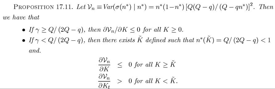
This proposition establishes that the variability of growth in the economy will eventual ly decline (and in fact disappear). But one might wish to know whether the amplitudes of eco­nomic fluctuations are systematically related to the level of the capital stock or output in the economy. This is particularly relevant, since, as already discussed, both cross-sectional and time-series comparisons suggest that poorer nations suffer from greater economic variability. To answer this question, the natural variable to look at is the conditional variance of TFP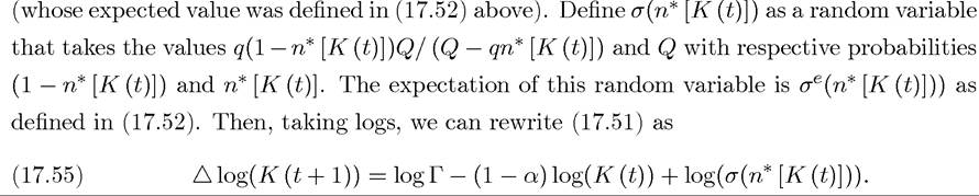

It is clear from this equation that capital (and output) growth volatility, after removing the deterministic “convergence effects” due to the standard neoclassical effects, are determined by the stochastic component σ. Denoting the (conditional) variance of σ(n* [K (t)] given K (t) by V_n, we can state the following proposition.

Proof. See Exercise 17.28. ?

The behavior of the variability of growth in this proposition results from the counteract­ing effects of two forces; first, as the economy develops, more savings are invested in risky assets; and second, as more sectors are opened, idiosyncratic risks are better diversified. The proposition shows that ifthe second effect always dominates and thus the

richer economies are less risky. Ifthen the first effect dominates for suf­

ficiently low levels of capital stock but once the capital stock reaches a critical threshold, K, the second effect again dominates. Thus except for sufficiently low levels of capital, the variability of the growth rate is everywhere decreasing in the income (or capital) level of the economy.

17.6.4. Efficiency. The previous subsection completely characterized the stochastic equilibrium of the economy. Is this equilibrium Pareto efficient? Since all agents are price takers, it may be conjectured that the answer to this question must be yes. In this subsection I show that this is not the case. Though at first surprising, this result will turn out to be intu­itive and interesting. First, it results from an economically meaningful pecuniary externality. Second, it makes sense from the viewpoint of the theory of general equilibrium; though all agents are price takers, this is not an Arrow-Debreu economy because the set of traded com­modities is determined endogenously by a zero profit condition. To illustrate these issues in the most transparent way I ignore any potential source of intertemporal inefficiency (which, we know from Chapter 9, may arise in overlapping generations economies). For this reason, the analysis of efficiency takes a particular level of savings s (t), or equivalently the current level of the capital stock K (t), as given and looks at whether the way in which savings are allocated across different sectors of the economy is (constrained) efficient. We do this, by 684

More specifically, the social planner chooses the set of sectors that are active, which is denoted

by [0,n (t)], the amount that will be invested in the safe sector X (t) and the allocation of funds among the other sectors denoted byIn principle, the social planner

could have chosen the set of active sectors not to be an interval of the form [0,n (t)], but the same argument as in Exercise 17.24 ensures that there is no loss of generality in imposing this form. The constraint makes sure that the sum of investments in the safe and the risky sectors

is less than the amount of savings available to the planner. The main difference between this program and the maximization problem of the representative household (17.40) is that the social planner also chooses n (t), while the representative household took the set of available assets as given. The social planner’s allocation (and thus the Pareto optimal allocation) is given by the solution to this maximization problem. The next proposition characterizes the

solution.

Proposition 17.12. Let n* [K (t)] be given by (17.50), and s (t) and K (t) denote current level of savings and capital stock available to the social planner. Then, the unique solution to the maximization problem in (17.56) is as follows:

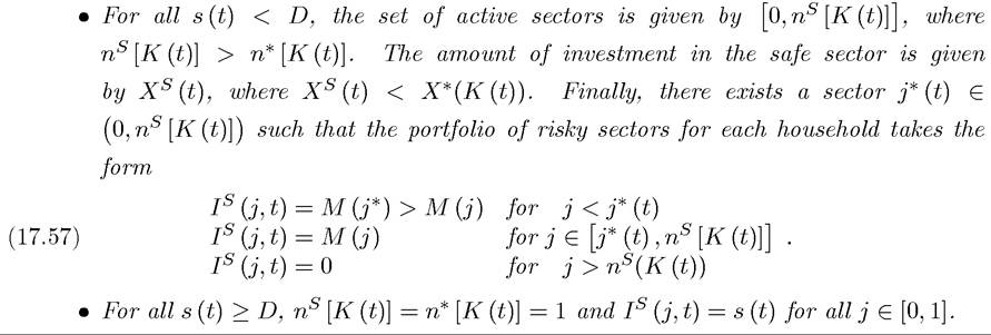
Proof. See Exercise 17.29. ?

This proposition implies that, when the economy has not achieved full diversification, the social planner will open more sectors than the decentralized equilibrium. She will finance these additional sectors by deviating from the balanced portfolio, which was always a feature of the equilibrium allocation. In other words, she will invest less in the sectors without the minimum size requirement. The Pareto optimal allocation of funds is shown in Figure 17.5.

685

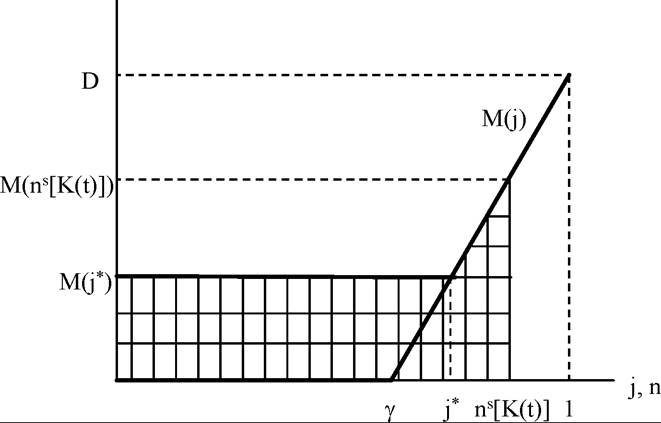
Figure 17.5. The efficient portfolio allocation.

The deviation from the balance portfolio implies that the social planner is implicitly cross­subsidizing the sectors with high a minimum size requirements at the expense of sectors with low or no minimum size requirements. This is because, starting with a balanced portfolio, opening a few more sectors always benefits consumers, who will be able to achieve better risk diversification. The only way the social planner can achieve this is by implicitly taxing sectors that have low or no minimum size requirements (so that they have high Lagrange multipliers and thus lower investments) and subsidizing the marginal sectors with high minimum size requirements.

Why does the decentralized equilibrium not achieve the same allocation? There are two complementary ways of providing the intuition for this. The first is that a marginal dollar of investment by an household in a high minimum size requirements sector creates a pecuniary externality, because this investment makes it possible for the sector to be active and thus provide better risk diversification possibilities to all the other agents. However, each household, taking equilibrium prices as given, ignores this pecuniary externality and tends to underinvest in marginal sectors with high minimum size requirements. Thus the source of inefficiency is that each household ignores its impact on others’ diversification opportunities. The second intuition for this result is related. Because households take the set of prices as given and in equilibrium P (j, t) = 1 for all active sectors, they will always hold a balanced portfolio. However, the Pareto optimal allocation involves cross-subsidization across sectors 686

in a non-balanced portfolio. Market prices do not induce the households to hold the right portfolio.

At this point, the reader may wonder why the First Welfare Theorem does not apply. In particular, all households are price takers. The reason why the First Welfare Theorem does not apply that the decentralized equilibrium here does not correspond to an Arrow- Debreu equilibrium. In particular, this is an equilibrium for an economy with endogenously incomplete markets, where the set of active markets is determined by zero profit (free entry) condition. All commodities that are traded in equilibrium are priced competitively but there is no “competitive pricing” for commodities that are not traded. Instead, in an Arrow- Debreu equilibrium, all commodities, even those that are not traded in equilibrium, are priced and in fact a potential commodity would not be traded in equilibrium only if its price were equal to numeral a zero and at zero prices generated excess supply. In this sense, the equilibrium characterized here is not an Arrow-Debreu equilibriumand in fact such an equilibrium does not exist in this economy because of the nonconvexity in the production set. Instead, the equilibrium concept used here is a more natural competitive equilibrium notion, which requires that all commodities that are traded in equilibrium are priced competitively and then determines the set of traded commodities by a free entry condition. Some additional discussion of this equilibrium concept is provided in the References and Literature section below

17.6.5. Inefficiency with Alternative Market Structures. Would the market fail­ure in portfolio choices be overcome if some financial institution could coordinate households’ investment decisions? Imagine that rather than all agents acting in isolation and ignoring their impact on each others’ decisions, funds are intermediated through a financial coalition­intermediary. This intermediary can collect all the savings and offer to each saver a complex security (as different from a Basic Arrow Security) that paysin each state

and X^s (t) are as in the optimal portfolio. Holding this security would make each consumer better off compared to the equilibrium.

Although from this discussion it may appear that the inefficiency we identified may not be robust to the formation of more complex financial institutions, we will show that this is not the case. The remarkable result is that unless some rather strong assumptions are made about the set of contracts that a financial intermediary can offer, equilibrium allocations resulting from competition among intermediaries will be identical to the equilibrium allocation in Proposition 17.8. A full analysis of this issue is beyond the scope of the current book, but a brief discussion gives the flavor. Let us model more complex financial intermediaries as “intermediary-coalitions,” that is, as a set of households who join their savings together and invest in a particular portfolio intermediate sectors. Such coalitions may be organized by 687

a specific household, and if it is profitable for other households to join the coalition, the organizer of the coalition can charge a premium (or a joining fee) thus making profits. We assume that there is free entry into financial intermediation or coalition-building, so that any household can attempt to exploit profit opportunities if there are any. Let us also impose some structure on how the timing of financial intermediation works and also how individual households can participate into different coalitions. In particular, let us adopt the following assumptions.

(1) Coalitions maximize a weighted utility of their members at all points in time. In particular, a coalition cannot commit to a path of action that will be against the interests of its members in the continuation game.

(2) Coalitions cannot exclude other agents (or coalitions) from investing in a particular pro ject.

Acemoglu and Zilibotti (1997) prove the following result.

Proposition 17.13. The set of equilibria of the financial intermediation game described above is always non-empty and all equilibria have exactly the same structure as those char­acterized in subsection 17.6.2 and Proposition 17.8.

I will not provide a proof of this proposition, since a formal statement of the proposition and the proof require additional notation. But the intuition is straightforward: as shown in Proposition 17.12, the Pareto optimal allocation involves a non-balanced portfolio and cross­subsidization across different sectors. This implies that the shadow price of investing in some sectors should be higher than in others, even though the cost of investing in each sector is equal to 1 (terms of date t final goods). These differences in shadow prices will then support a non-balanced portfolio. Recall also that it is the sectors with no minimum size requirement or low minimum size requirements that are being implicitly taxed in this allocation. This kind of cross-subsidization is difficult to sustain in equilibrium because each household would deviate towards slightly reducing its investments in coalitions/intermediaries that engage in cross-subsidization and undertake investments on the side to move its portfolio towards a balanced one (by investing in no minimum size or low minimum size sectors). At the end, only allocations without cross-subsidization can survive as equilibria, and those are identical to equilibria characterized in subsection 17.6.2.

The most important implication of this result is that even with unrestricted financial intermediaries or coalitions, the inefficiency resulting from endogenously incomplete markets cannot be prevented. The key economic force is that each household creates a positive pecuniary externality by holding a non-balanced portfolio but in a decentralized equilibrium each household wishes to and can easily move towards a balanced portfolio, undermining efforts to sustain the efficient allocation.

17.7.