Schooling Investments and Returns to Education

We now turn to the simplest model of schooling decisions in partial equilibrium, which will illustrate the main tradeoffs in human capital investments. The model presented here is a version of Mincer’s (1974) seminal contribution.

Let us first assume that T = ∞, which will simplify the expressions. The flow rate of death, ν, is positive, so that individuals have finite expected lives. Suppose that (10.2) is such that the individual has to spend an interval S with s (t) = 1—i.e., in full-time schooling, and s (t) = 0 thereafter. At the end of the schooling interval, the individual will have a schooling level of

where η (∙) is an increasing, continuously differentiable and concave function. For t ∈ [S, ∞), human capital accumulates over time (as the individual works) according to the differential equation

⁽id="Picutre 1235" class="lazyload" data-src="/files/uch_group77/uch_pgroup317/uch_uch7364/image/image1233.jpg">

for some gh ≥ 0. Suppose also that wages grow exponentially,

⁽

with boundary condition w (0) > 0.

Suppose that

so that the net present discounted value of the individual is finite. Now using Theorem 10.1, the optimal schooling decision must be a solution to the following maximization problem

Now using (10.6) and (10.7), this is equivalent to (see Exercise 10.3):

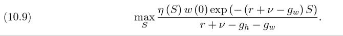
Since η (S) is concave, the objective function in (10.9) is strictly concave.

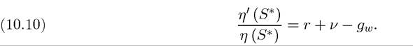
Equation (10.10) shows that higher interest rates and higher values of ν (corresponding to shorter planning horizons) reduce human capital investments, while higher values of g_w increase the value of human capital and thus encourage further investments.

386

Integrating both sides of this equation with respect to S, we obtain

Now note that the wage earnings of the worker of age τ ≥ S* in the labor market at time t will be given by

Taking logs and using equation (10.11) implies that the earnings of the worker will be given by

where t — S can be thought of as worker experience (time after schooling). If we make a cross-sectional comparison across workers, the time trend term g_wt, will also go into the constant, so that we obtain the canonical Mincer equation where, in the cross section, log wage earnings are proportional to schooling and experience. Written differently, we have the following cross-sectional equation

where j refers to individual j. Note however that we have not introduced any source of heterogeneity that can generate different levels of schooling across individuals. Nevertheless, equation (10.12) is important, since it is the typical empirical model for the relationship between wages and schooling estimated in labor economics.

The economic insight provided by this equation is quite important; it suggests that the functional form of the Mincerian wage equation is not just a mere coincidence, but has eco­nomic content: the opportunity cost of one more year of schooling is foregone earnings.

As already discussed in Chapter 3, empirical work using equations of the form (10.12) leads to estimates for γ in the range of 0.06 to 0.10. Equation (10.12) suggests that these returns to schooling are not unreasonable. For example, we can think of the annual interest rate r as approximately 0.10, ν as corresponding to 0.02 that gives an expected life of 50 years, and g_w corresponding to the rate of wage growth holding the human capital level of the individual constant, which should be approximately about 2%. Thus we should expect an estimate of γ around 0.10, which is consistent with the upper range of the empirical estimates.

10.3.