The Ben-Porath Model
The baseline Ben-Porath model enriches the model studied in the previous section by allowing human capital investments and non-trivial labor supply decisions throughout the 387
lifetime of the individual.
In particular, we now let s (t) ∈ [0,1] for all t ≥ 0. Together with the Mincer equation (10.12) (and the model underlying this equation presented in the previous section), the Ben-Porath model is the basis of much of labor economics. Here it is sufficient to consider a simple version of this model where the human capital accumulation equation, (10.2), takes the form
where δ}l > 0 captures “depreciation of human capital,” for example because new machines and techniques are being introduced, eroding the existing human capital of the worker. The individual starts with an initial value of human capital h (0) > 0. The function φ :
strictly increasing, continuously differentiable and strictly concave. Furthermore, we simplify the analysis by assuming that this function satisfies the Inada-type conditions,
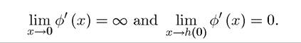
The latter condition makes sure that we do not have to impose additional constraints to ensure s (t) ∈ [0,1] (see Exercise 10.5).
Let us also suppose that there is no non-human capital component of labor, so that ω (t) = 0 for all t, that T = ∞, and that there is a flow rate of death v > 0. Finally, we assume that the wage per unit of human capital is constant at w and the interest rate is constant and equal to r. We also normalize w = 1 without loss of any generality.
Again using Theorem 10.1, human capital investments can be determined as a solution to the following problem
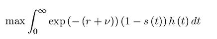
subject to (10.13).
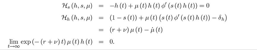
This problem can be solved by setting up the current-value Hamiltonian, which in this case takes the form

where we used H to denote the Hamiltonian to avoid confusion with human capital. The necessary conditions for this problem are
388
To solve for the optimal path of human capital investments, let us adopt the following transformation of variables:
Instead of s (t) (or μ (t)) and h (t), we will study the dynamics of the optimal path in x (t) and h (t).
The first necessary condition then implies that

while the second necessary condition can be expressed as
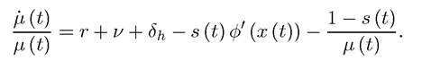
Substituting for μ (t) from (10.14), and simplifying, we obtain

The steady-state (stationary) solution of this optimal control problem involves μ (t) = 0 and h (t) = 0, and thus implies that

where is the inverse function oi
 (which exists and is strictly decreasing since φ (∙) is strictly concave). This equation shows that
 will be higher when the interest rate
is low, when the life expectancy of the individual is high, and when the rate of depreciation of human capital is low.
To determine s* and h* separately, we set h (t) = 0 in the human capital accumulation equation (10.13), which gives
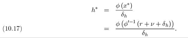
Since (∙) is strictly decreasing and φ (∙) is strictly increasing, this equation implies that the steady-state solution for the human capital stock is uniquely determined and is decreasing in r, ν and δ⅛.
More interesting than the stationary (steady-state) solution to the optimization problem is the time path of human capital investments in this model. To derive this, differentiate (10.14) with respect to time to obtain

389
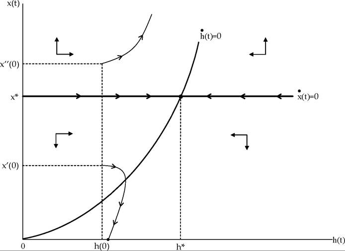
FIGURE 10.1. Steady state and equilibrium dynamics in the simplified Ben Porath model.
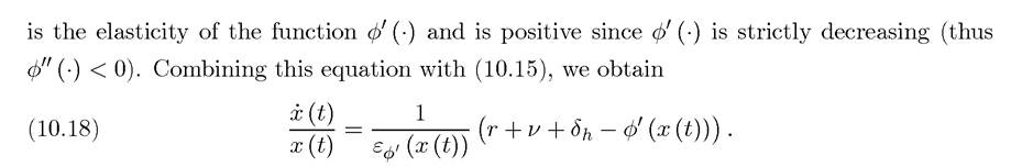
Figure 10.1 plots (10.13) and (10.18) in the h-x space. The upward-sloping curve corresponds to the locus for h (t) = 0, while (10.18) can only be zero at x*, thus the locus for corresponds to the horizontal line in the figure. The arrows of motion are also plotted in this phase diagram and make it clear that the steady-state solution (h*,x*) is globally saddle-path stable, with the stable arm coinciding with the horizontal line for
 Starting with h (0) ∈ (0,h*), s (0) jumps to the level necessary to ensure s (0) h (0) = x*. From then on, h (t) increases and s (t) decreases so as to keep s (t) h (t) = x*. Therefore, the pattern of human capital investments implied by the Ben-Porath model is one of high investment at the beginning of an individual’s life followed by lower investments later on.
In our simplified version of the Ben-Porath model this all happens smoothly. In the original Ben-Porath model, which involves the use of other inputs in the production of human capital and finite horizons, the constraint for s (t) ≤ 1 typically binds early on in the life of the individual, and the interval during which s (t) = 1 can be interpreted as full-time 390
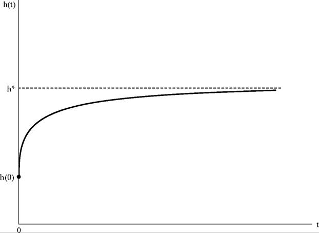
Figure 10.2. Time path of human capital investments in the simplified Ben Porath model.
schooling. After full-time schooling, the individual starts working (i.e., s (t) < 1). But even on-the-job, the individual continues to accumulate human capital (i.e., s (t) > 0), which can be interpreted as spending time in training programs or allocating some of his time on the job to learning rather than production. Moreover, because the horizon is finite, if the Inada conditions were relaxed, the individual could prefer to stop investing in human capital at some point. As a result, the time path of human capital generated by the standard Ben-Porath model may be hump-shaped, with a possibly declining portion at the end (see Exercise 10.6). Instead, the path of human capital (and the earning potential of the individual) in the current model is always increasing as shown in Figure 10.2.
The importance of the Ben-Porath model is twofold. First, it emphasizes that schooling is not the only way in which individuals can invest in human capital and there is a continuity between schooling investments and other investments in human capital. Second, it suggests that in societies where schooling investments are high we may also expect higher levels of on-the-job investments in human capital. Thus there may be systematic mismeasurement of the amount or the quality human capital across societies.
10.4.