Solving the Log-Linear Stochastic Growth Model

The model consists of equations (13.46), (13.49), (13.51), (13.52), (13.53), and (13.54). It determines fluctuations around the steady state for output, the capital stock, consumption, employment, the real interest, and the real wage.

We can first solve the subsystem of (13.49), (13.52), and (13.54) for capital, employment, and consumption, and then substitute in the other three equations to determine output, the real interest rate, and the real wage.

The easiest way to solve the model analytically is to use the method of undetermined coefficients. We start from the equation for consumption and conjecture that consumption will be a linear function of the two state variables k and a, of the form

where η_CK and η_CA are coefficients to be determined. Substituting (13.56) in the employment equation (13.54), we get the solution for employment as

where η_LK = να − η_CK, and η_LA = 1 − α − η_CA.

Substituting (13.56) and (13.57) in the capital accumulation equation (13.49), and making use of the exogenous process (13.55), we get the solution for the accumulation of capital:

where

Finally, we can substitute (13.57) and (13.58) in the Euler equation for consumption (13.52) and take the rational expectations solution, using the exogenous process (13.55) as well.

Comparing coefficients between (13.59) and (13.56), we can determine the undetermined coefficients η_CK and η_CA.

13.4.1 Aggregate Fluctuations around the Steady State

We can now use the solution obtained to characterize the fluctuations of the various aggregates around the steady state. From (13.58) and (13.55), fluctuations in the capital stock are determined by

Logarithmic deviations of the capital stock from its steady state value follow a stationary AR(2) process.

Substituting (13.60) and (13.55) in the consumption equation (13.56), we can see that log deviations of consumption from its steady state follow a stationary autoregressive-moving average, process ARMA(2,1). This takes the form

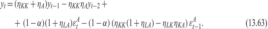
Substituting (13.60) and (13.55) in the employment equation (13.57), we have that log deviations of employment from its steady state follow a stationary ARMA(2,1) process of the form

alt=eq13-62.png>

Finally, substituting (13.60) and (13.61) in the log-linear version of the aggregate production function (13.46), log deviations of output from its steady state follow:

Thus, log deviations of output from its steady state follow an ARMA(2, 1) process as well.

13.4.2 A Dynamic Simulation of the Log-Linear Stochastic Growth Model

Figure 13.1 presents the results of a dynamic simulation of the model for a 1% positive shock to productivity a. The parameter values used in the simulation were α = 0.333, ρ = 0.02, g = 0.02, δ = 0.03, ν = 2, and η_A = 0.90. As can be seen from the simulated impulse response functions, all real variables move procyclically, as innovations in productivity affect output, the capital stock, consumption, and employment in the same direction. Real wages and the real interest rate also move procyclically. Gradually, all variables converge to their original steady state values, unless the system is disturbed by another shock.

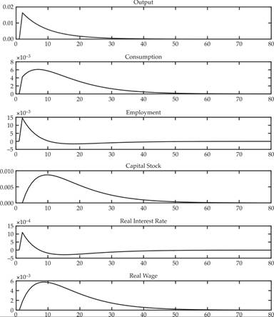
Figure 13.1 Dynamic simulation of the stochastic growth model following a 1% persistent shock to productivity.

Thus, the general stochastic growth model can explain fluctuations in all real variables as a result of stochastic shocks to productivity. However, fluctuations in employment are due to intertemporal substitution in labor supply, and there is no account for unemployment.

13.5