A Log-Linear Approximation to the General Stochastic Growth Model
In this section, we proceed to analyze the general version of the stochastic growth model without some of the more extreme simplifications introduced in section 13.2. We set out the full stochastic growth model and derive an approximate analytical solution, based on a log-linear approximation around the steady state equilibrium.
Following Campbell [1994], the model is thus transformed into a system of log-linear stochastic difference equations, which can be solved by the method of undetermined coefficients. We solve the model assuming that government expenditure is equal to zero.The first equation of the stochastic growth model is the production function

where 0 < α < 1.
The second equation is the capital accumulation process:

The representative household maximizes

subject to the accumulation process (13.35). Finally, there is a representative perfectly competitive firm that maximizes profits subject to the production function (13.34).
From the first-order conditions for profit maximization, the marginal product of capital and labor are equal to the real interest rate and the real wage, respectively. It thus follows that
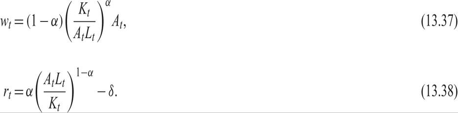
From the first-order conditions for the maximization of the utility of the representative household, it also follows that
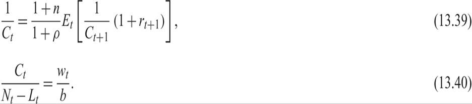
Equation (13.39) is a stochastic version of the Euler equation for aggregate consumption, and (13.40) relates current consumption and leisure to the real wage.
13.3.1 The Steady State
In the steady state, aggregate variables such as output, effective labor, capital, and consumption grow at an exogenous rate g + n. Thus, from (13.39), the steady state real interest rate is determined by the condition

Equation (13.41) implies that

From the marginal productivity condition for capital (13.38), the steady state ratio of output to capital is determined by

From (13.43), the steady state ratio of effective labor to capital is determined by
alt=eq13-44.png>
Finally, from the capital accumulation process (13.35) and (13.43), the steady state consumption to output ratio is given by

Note that the last term in (13.45) is the steady state savings rate.
13.3.2 Log-Linearizing the Model around the Steady State
Let us consider fluctuations of the endogenous variables around the steady state. Outside the steady state, the model is a system of nonlinear equations in the logs of productivity, capital, labor, output, and consumption. Nonlinearities arise because of the depreciation rate, the equation for capital accumulation, the variable savings rate, and the variable employment rate. Unlike the simplified version of the model that we examined in section 13.2, which could be solved fully, let us seek an approximate analytical solution by taking a log-linear approximation of all equations around the steady state.
The Cobb-Douglas production function can be log-linearized directly. From (13.34), it follows that

where lowercase letters denote the difference of the logarithm of the relevant variable from its steady state value.
The capital accumulation equation (13.35) is obviously not log-linear. Dividing by Kt, it can be written as

Taking logs, (13.47) can be written as

Taking a first-order Taylor approximation of (13.48) around the steady state and using the log-linear version of the production function (13.46), we end up with the following log-linear approximation of the accumulation equation around the steady state:

where  , and
, and  .
.
We next turn to the determination of the real interest rate and the Euler equation for consumption. From the marginal productivity condition for capital, (13.38), it follows that

Taking a log-linear approximation of (13.50) around the steady state, we get

where  . Substituting (13.51) in the Euler equation for consumption (13.39) and assuming that the variables on the right-hand side are jointly log-normal, the Euler equation for consumption can be written as

Log-linearizing the marginal productivity condition for labor (13.37) and taking deviations from steady state, we get that deviations of the log of the real wage from steady state are given by

Finally, log-linearizing the first-order condition for consumption and leisure (13.40) and using the marginal productivity condition for employment (13.53) to substitute for the logarithm of the real wage, we get

where 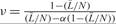 .
.
 is steady state labor supply as a fraction of total available time. Following Prescott [1986], let us assume that this is equal to about one-third.
 To close the model, we need only specify the exogenous stochastic process driving productivity a. Let us continue to assume, as in section 13.2, that it follows an AR(1) process of the form

where 0 < ηA < 1.
13.4
More on the topic A Log-Linear Approximation to the General Stochastic Growth Model:
- The Stochastic Growth Model
- Alogoskoufis George. Dynamic Macroeconomics. The MIT Press,2019. — 800 p., 2019
- Contents
- A Simplified Version of the Stochastic Growth Model
- Solow Model and Regression Analyses
- Solow Model and Regression Analyses