The Lab Equipment Model of Growth with Input Varieties

We start with a particular version of the endogenous growth model with expanding vari­eties of inputs and an R&D technology that only uses output for creating new inputs. This is sometimes referred to as the lab equipment model, since all that is required for research is in­vestment in equipment or in laboratories—rather than the employment of skilled or unskilled workers or scientists.

13.1.1.

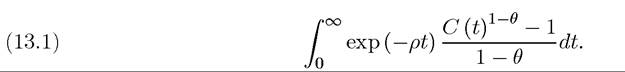
There is no population growth, and the total population of workers, L, supplies labor inelas- tically throughout. We also assume, as discussed in the previous chapter, that the represen­tative household owns a balanced portfolio of all the firms in the economy. Alternatively, we can think of the economy as consisting of many households with the same preferences as the representative household and each household holding a balanced portfolio of all the firms.

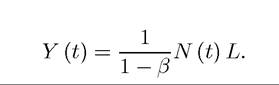
The unique consumption good of the economy is produced with the following aggregate production function:

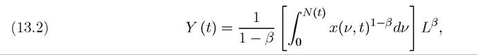
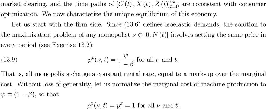
where L is the aggregate labor input, N (t) denotes the different number of varieties of inputs (machines) available to be used in the production process at time t, and x (ν, t) is the total amount of input (machine) type ν used at time t. We assume that x’s depreciate fully after use, thus they can be interpreted as generic inputs, as intermediate goods, as machines, or even as capital as long as we are comfortable with the assumption that there is immediate depreciation. The assumption that the inputs or machines are “used up” in production or depreciate immediately after being used makes sure that the amounts of inputs used in the past do not become additional state variables, and simplifies the exposition of the model (though the results are identical without this assumption, see Exercise 13.22).

The term (1 — β) in the denominator is included for notational simplicity. Notice that for given N(t), which final good producers take as given, equation (13.2) exhibits constant returns to scale. Therefore, final good producers are competitive and are subject to constant returns to scale, justifying our use of the aggregate production function to represent their production possibilities set.

One can also write (13.2) in the following form

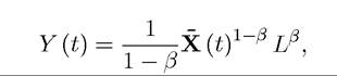
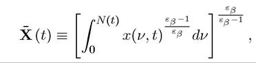
where

474

with εβ ? 1∕β as the elasticity of substitution between inputs. This form emphasizes both the constant returns to scale properties of the production function and the continuity between the model here and the Dixit-Stiglitz model of the previous chapter.

The resource constraint of the economy at time t is where X (t) is investment or spending on inputs at time t and Z (t) is expenditure on R&D at time t, which comes out of the total supply of the final good.

We next need to specify how quantities of machines are created and how new machines are invented. Let us first assume that once the blueprint of a particular input is invented, the research firm can create one unit of that machine at marginal cost equal to ψ > 0 units of the final good. We also assume the following form for innovation possibilities frontier, where new machines are created as follows:

where η > 0, and the economy starts with some initial technology stock N (0) > 0. This implies that greater spending on R&D leads to the invention of new machines.

There is no aggregate uncertainty in the innovation process. Naturally, there will be un­certainty at the level of the individual firm, but with many different research labs undertaking such expenditure, at the aggregate level, equation (13.4) holds deterministically.

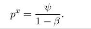
Given the patent structure specified above, a firm that invents a new machine variety is the sole supplier of that type of machine, say machine of type ν, and sets a price of at time t to maximize profits. Since machines depreciate after use,can also be interpreted as a “rental price” or the use and cost of this machine.

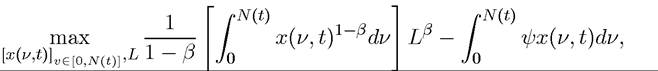
The demand for machine of type ν is obtained by maximizing net aggregate profits of the final good sector as given by (13.2) minus the cost of inputs. Since machines depreciate after use and labor is hired on the spot market for its flow services, the maximization problem on the final good sector can be considered for each point in time separately, and simply requires the maximization of the instantaneous profits of a representative final good producer. These instantaneous profits can be obtained by subtracting the total inputs costs, the user costs of renting machines and labor costs, from the value of our production. Therefore, the maximization problem at time t is:

The first-order condition of this maximization problem with respect to x (ν, t) for any yields the demand for machines from the final good sector.

which is intuitive in view of the fact that elasticity of demand for different machine varieties This equation implies that the demand for machines only depends on the user cost of the machine and on equilibrium labor supply but not on the interest rate, r (t), the wage rate, w (t), or the total measure of available machines, N (t). This feature makes the model very tractable.

Now consider the maximization problem of a monopolist owning the blueprint of a ma­chine of type ν invented at time t. Since the representative household holds a balanced portfolio of all the firms in the economy and there is a continuum of firms, there will be no aggregate uncertainty, so each monopolist’s objective is to maximize profits. Consequently, this monopolist chooses an investment plan and a sequence of capital stocks so as to maximize the present discounted value of profits starting from time t. Recalling that the interest rate at time t is r (t) and the marginal cost of producing machines (in terms of the final good) is ψ, the net present discounted value can be written as:

where π(ν, t) ? p^x(ν, t)x(ν, t) — ψx(ν, t) denotes profits of the monopolist producing inter­mediate ν at time t, x(ν, t) and p^x(ν, t) are the profit-maximizing choices for the monopolist, and r (t) is the market interest rate at time t. Alternatively, assuming that the value func­tion is differentiable in time, this could be written in the form of Hamilton-Jacobi-Bellman equations as in Theorem 7.10 in Chapter 7:

Exercise 13.1 asks you to provide a different derivation of this equation than in Theorem

7.10.

13.1.2. Characterization of Equilibrium. An allocation in this economy is defined by the following objects: time paths of consumption levels, aggregate spending on machines, and aggregate R&D expenditurtime paths of available machine

types, [N (t)]∞o, time paths of prices and quantities of each machine and the net present discounted value of profits from that machine,and time

paths of interest rates and wage rates,

An equilibrium is an allocation in which all existing research firms choose

to maximize profits, the evolution ofis determined by free entry, the time paths of interest rates and wage rates,are consistent with

Profit-maximization also implies that each monopolist rents out the same quantity of ma­chines in every period, equal to

This gives monopoly profits as:

The important implication of this equation is that each monopolist sells exactly the same amount of machines, charges the same price and makes the same amount of profits at all time points. This particular feature simplifies the analysis of endogenous technological change models with expanding variety.

Substituting (13.6) and the machine prices into (13.2) yields a final good production function of the form

(13.12)

This is one of the main equations of the expanding product or input variety models.

The labor demand of the final good sector follows from the first-order condition of max­imizing (13.5) with respect to L and implies the equilibrium condition

(13.13)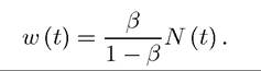

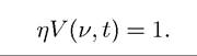
Finally, free entry into research implies that at all points in time we must have

where V(ν, t) is given by (13.7). To understand (13.14), recall that one unit of final good spent on R&D leads to the invention of η units of new inputs, each with a net present discounted value of profits given by (13.7). This free entry condition is written in the complementary slackness form, since research may be very unprofitable and there may be zero R&D effort, in which case ηV(ν, t) could be strictly less than 1. Nevertheless, for the relevant parameter values there will be positive entry and economic growth (and technological progress), so we often simplify the exposition by writing the free-entry condition as

Note also that since each monopolist ν ∈ [0,N(t)] produces machines given by (13.10), and there are a total of N (t) monopolists, the total expenditure on machines is

Finally, the representative household’s problem is standard and implies the usual Euler equa­tion:

1555" class="lazyload" data-src="/files/uch_group77/uch_pgroup317/uch_uch7364/image/image1553.jpg">

and the transversality condition

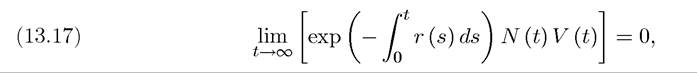
which is written in the “market value” form and requires the value of the total wealth of the representative household, which is equal to the value of corporate assets N (t) V (t), not to grow faster than the discount rate (see Exercise 13.3).

In light of the previous equations, we can now define an equilibrium more formally as 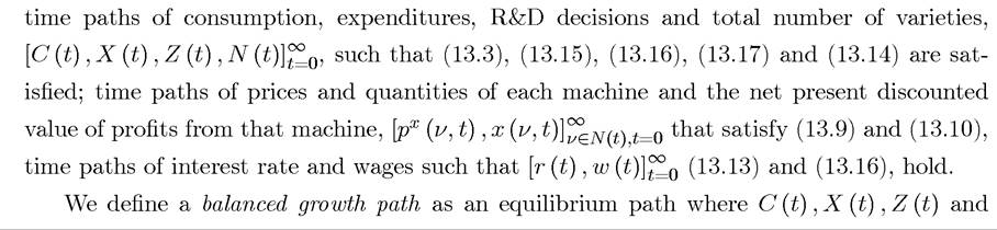N (t) grow at a constant rate. Such an equilibrium can alternatively be referred to as a “steady state”, since it is a steady state in transformed variables (even though the original variables grow at a constant rate). This is a feature of all the growth models and we will throughout use the terms steady state and balanced growth path interchangeably when referring to endogenous growth models.

13.1.3. Balanced Growth Path. A balanced growth path (BGP) requires that con­sumption grows at a constant rate, say gc. This is only possible from (13.16) if the interest 478

rate is constant. Let us therefore look for an equilibrium allocation in which

whererefers to BGP values. Since profits at each date are given by (13.11) and since the interest rate is constant, (13.8) implies thatSubstituting this in either (13.7) or

(13.8), we obtain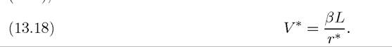

This equation is intuitive: a monopolist makes a flow profit of βL, and along the BGP, this is discounted at the constant interest rate r*.

Let us next suppose that the (free entry) condition (13.14) holds as an equality, in which case we also have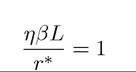

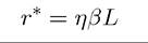
This equation pins down the steady-state interest rate, r*, as:

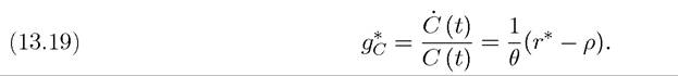
The consumer Euler equation, (13.16), then implies that the rate of growth of consumption must be given by

Moreover, it can be verified that the current-value Hamiltonian for the consumer’s maxi­mization problem is concave, thus this condition, together with the transversality condition, characterizes the optimal consumption plans of the consumer.

In a balanced growth path, consumption cannot grow at a different rate than total output (see Exercise 13.5), thus we must also have the growth rate of output in the economy is

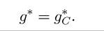
Therefore, given the BGP interest rate we can simply determine the long-run growth rate of the economy as:

We next assume that

which will ensure thatand that the transversality condition is satisfied.

We then obtain:

Proposition 13.1. Suppose that condition (13.21) holds. Then, in the above-described lab equipment expanding input variety model, there exists a unique balanced growth path in which technology, output and consumption all grow at the same rate, g*, given by (13.20).

Proof. The preceding discussion establishes all the claims in the proposition except that the transversality condition holds. You are asked to check this in Exercise 13.7. ?

An important feature of this class of endogenous technological progress models is the presence of the scale effect, which we encountered in Section 11.4 in Chapter 11: the larger is L, the greater is the growth rate. The scale effect comes from a very strong form of the market size effect discussed in the previous chapter. As illustrated there, the increasing returns to scale nature of the technology (for example, as highlighted in equation (13.12)) is responsible for this strong form of the market size effect and thus for the scale effect. We will see in Section 15.5 in Chapter 15 that it is possible to have variants of the current model that feature the market size effect, but not the scale effect.

13.1.4. Transitional Dynamics. It is also straightforward to see that there are no transitional dynamics in this model. To derive this result, let us go back to the value function for each monopolist. Substituting for profits, this gives

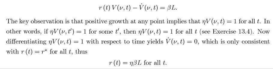
This establishes:

Proposition 13.2. Suppose that condition (13.21) holds. In the above-described lab equipment expanding input-variety model, with initial technology stock N (0) > 0, there is a unique equilibrium path in which technology, output and consumption always grow at the rate g* as in (13.20).

At some level, this result is not too surprising. While the microfoundations and the eco­nomics of the expanding varieties model studied here are very different from the neoclassical AK economy, the mathematical structure of the model is very similar to the AK model (as most clearly illustrated by the derived equation for output, (13.12)). Consequently, as in the AK model, the economy always grows at a constant rate.

Even though the mathematical structure of the model is similar to the neoclassical AK economy, it is important to emphasize that the economics here is very different. The equilib­rium in Proposition 13.2 exhibits endogenous technological progress. In particular, research firms spend resources in order to invent new inputs. They do so because, given their patents, they can profitably sell these inputs to final good producers. It is therefore profit incentives 480

that drive R&D, and R&D drives economic growth. We have therefore arrived to our first model in which market-shaped incentives determine the rate at which the technology of the economy evolves over time.

13.1.5. Pareto Optimal Allocations. The presence of monopolistic competition im­plies that the competitive equilibrium is not necessarily Pareto optimal. In particular, the current model exhibits a version of the aggregate demand externalities discussed in the pre­vious chapter and features two sources of potential inefficiencies. First, there is a markup over the marginal cost of production of inputs. Second, the number of inputs produced at any point in time may not be optimal. The first source of inefficiency is familiar from models of static monopoly, while the second emerges from the fact that in this economy the set of traded (Arrow-Debreu) commodities is endogenously determined. This latter source of po­tential inefficiency relates to the issue of endogenously incomplete markets (there is no way to purchase an input that is not supplied in equilibrium) and will be discussed in greater detail in Section 17.6 in Chapter 17.

To contrast the equilibrium allocations with the Pareto optimal allocations, we set up the problem of the social planner and derive the optimal growth rate. Notice that the social planner will also use the same quantity of all types of machines in production, but because of the absence of a markup, this quantity will be different than in the equilibrium allocation. The social planner will also take into account the effect of an increase in the variety of inputs on the overall productivity in the economy, which monopolists did not because they did not appropriate the full surplus from inventions.

More explicitly, given N (t), the social planner will choose

which only differs from the equilibrium profit maximization problem, (13.5), because the marginal cost of machine creation, ψ, is used as the cost of machines rather than the monopoly price, and the cost of labor is not subtracted. Recalling that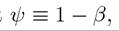the solution to this

program involves

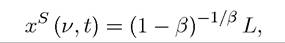
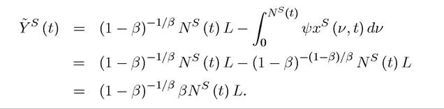
so that the social planner’s output level will be

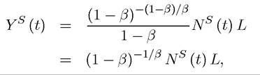
where superscripts “S” are used to emphasize that the level of technology and thus the level of output will differ between the social planner’s allocation and the equilibrium allocation.

481

The aggregate resource constraint is still given by (13.3). Let us define net output, which subtracts the cost of machines from total output, as

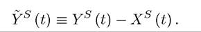
This is relevant, since it is net output that will be distributed between R&D expenditure and consumption. We obtain

Given this and (13.4), the maximization problem of the social planner can be written as

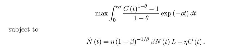
In this problem, N (t) is the state variable, and C (t) is the control variable. Let us set up the current-value Hamiltonian

The necessary conditions are

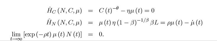
It can be verified easily that the current-value Hamiltonian of the social planner is concave, thus the necessary conditions are also sufficient for an optimal solution.

Combining these necessary conditions, we obtain the following growth rate for consump­tion in the social planner’s allocation (see Exercise 13.9):

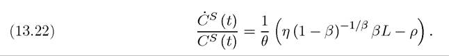
Like the equilibrium, the social planner also chooses and allocation with a constant rate of consumption growth (thus no transitional dynamics). The growth rate of consumption chosen by the social planner, (13.22), can be directly compared to the growth rate in the decentralized equilibrium, (13.20). The comparison boils down to that of

482

and it is straightforward to see that the former is always greater sinceby

virtue of the fact that β ∈ (0,1). This implies that the socially-planned economy will always grow faster than the decentralized economy

PROPOSITION 13.3. In the above-described expanding input variety model, the decentral­ized equilibrium is always Pareto suboptimal. Starting with any N (0) > 0, the Pareto optimal allocation involves a constant growth rate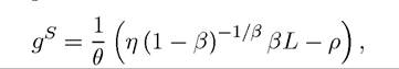 which is strictly greater than the equilibrium growth rate g* given in (13.20).

Proof. Most of the proof is provided in the preceding discussion. Exercise 13.11 asks you to show that the Pareto optimal allocation always involves a constant growth rate and no transitional dynamics. ?

Intuitively, the Pareto optimal growth rate is greater than the equilibrium growth rate because the social planner values innovation more. The greater social value of innovations stems from the fact that the social planner is able to use the machines more intensively after innovation, since the monopoly markup reducing the demand for machines is absent in the social planner’s allocation. This is related to the pecuniary externality resulting from the monopoly markups (and is thus related to the aggregate demand externalities discussed in the previous chapter) and also indirectly affects the set of traded commodities (thus the rate of growth of inputs and technology). Other models of endogenous technological progress we will study in this chapter incorporate technological spillovers and thus generate inefficiencies both because of the pecuniary externality isolated here and because of the standard technological spillovers.

13.1.6. Policy in Models of Endogenous Technological Progress. The divergence between the decentralized equilibrium and the socially planned allocation introduces the possibility of Pareto-improving policy interventions. There are two natural alternatives to consider:

(1) Subsidies to Research: by subsidizing research, the government can increase the growth rate of the economy, and this can be turned into a Pareto improvement if taxation is not distortionary and there can be appropriate redistribution of resources so that all parties benefit.

(2) Subsidies to Capital Inputs: inefficiencies also arise from the fact that the decentral­ized economy is not using as many units of the machines/capital inputs (because of the monopoly markup); so subsidies to capital inputs given to final good producers would also be useful in increasing the growth rate.

Moreover, it is noteworthy that as in the first-generation endogenous growth models, a variety of different policy interventions, including taxes on investment income and subsidies of various forms, will have growth effects not just level effects in this framework (see, for example, Exercise 13.13).

Naturally, once we start thinking of policy in order to close the gap between the decen­tralized equilibrium and the Pareto optimal allocation, we also have to think of the ob jectives of policymakers and this brings us to political economy issues, which are the sub ject matter of Part 8. For that reason, we will not go into a detailed discussion of optimal policy (leaving some of this to you in Exercises 13.12-13.14). Nevertheless, it is useful to briefly discuss the role of competition policy in models of endogenous technological progress.

Recall that the optimal price that the monopolist charges for machines is

Imagine, instead, that a fringe of competitive firms can copy the innovation of any monopolist, but they will not be able to produce at the same level of costs (because the inventor has more know-how). In particular, as in the previous chapter, suppose that instead of a marginal cost ψ, they will have marginal costthis fringe is not a threat

to the monopolist, since the monopolist could set its ideal, profit maximizing, markup and the fringe would not be able to enter without making losses. However,the

fringe would prevent the monopolist from setting its ideal monopoly price. In particular, in this case the monopolist would be forced to set a “limit price”, exactly equal to

This price formula follows immediately by noting that, if the price of the monopolist were higher than γψ, the fringe could undercut the price of the monopolist, take over to market and make positive profits. If it were below this, the monopolist could increase its price towards the unconstrained monopoly price and make more profits. Thus, there is a unique equilibrium price given by (13.23).

When the monopolist charges this limit price, its profits per unit would be

which is less than β, the profits per unit that the monopolist made in the absence of the competitive fringe.

What is the implication of this on the rate of economic growth? It is straightforward to work out that in this case the economy would grow at a slower rate. For example, in the baseline model with the lab-equipment technology, this growth rate would be (see Exercise 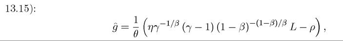484

which is less than g* given in (13.20). Therefore, in this model, greater competition, which reduces markups (and thus static distortions), also reduces long-run growth. This might at first appear counter-intuitive, since the monopoly markup may be thought to be the key source of inefficiency and greater competition (lower γ) reduces this markup. Nevertheless, as mentioned above, inefficiency results both because of monopoly markups and because the set of available inputs may not be appropriately chosen. As γ declines, monopoly markups decline, but the problem of underprovision of inputs becomes more severe. This is because profits are important in this model to encourage innovation by new research firms. If these profits are cut, incentives for research are also reduced. Since γ can also be interpreted as a parameter of anti-trust (competition) policy, this result implies that in the baseline endoge­nous technological change models more strict anti-trust policy reduces economic growth.

Welfare is not the same as growth, however, and some degree of competition reducing prices below the unconstrained monopolistic level might be useful for welfare depending on the discount rate of the representative household. Essentially, with a lower markup, households are happier in the present, but suffer slower consumption growth. The tradeoff between these two opposing effects depends on the discount rate of the representative household (see Exercise 13.15 for the details).

Similar results apply when we consider patent policy. In practice, patents are for limited durations. In the baseline model, we assumed that patents are perpetual; once a firm invents a new good, it has a fully-enforced patent forever and it becomes the monopolist for that good forever. If patents are enforced strictly, then this might rule out the competitive fringe from competing, restoring the growth rate of the economy to (13.20). Also, even in the absence of the competitive fringe, we can imagine that once the patent runs out, the firm will cease making profits on its innovation. In this case, it can easily be shown that growth is maximized by having as long patents as possible. Again there is a tradeoff here between the equilibrium growth rate of the economy and the static level of welfare.

Perhaps, more important than these tradeoffs between growth and level is the fact that the models discussed in this chapter do not feature an interesting type of competition among firms. The quality competition (Schumpeterian) models introduced in the next chapter will allow a richer analysis of the effect of competition on innovation and economic growth.

13.2.