Growth with Knowledge Spillovers
In the model of the previous section, growth resulted from the use of final output for R&D. This is similar, in some way, to the endogenous growth model of Rebelo (1991) we studied in Chapter 11, since the accumulation equation is linear in accumulable factors.
As a result, we saw that, in equilibrium, output took a linear form in the stock of knowledge (new machines), thus a AN form instead of Rebelo’s AK form.An alternative is to have “scarce factors” used in R&D. In other words, instead of the lab equipment specification, we now have scientists as the key creators of R&D. The lab equipment model generated sustained economic growth by investing more and more resources in the R&D sector. This is impossible with scarce factors, since, by definition, a sustained increase in the use of these factors in the R&D sector is not possible. Consequently, with this alternative specification, there cannot be endogenous growth unless there are knowledge spillovers from past R&D, making the scarce factors used in R&D more and more productive over time. In other words, we now need current researchers to “stand on the shoulder of past giants”. In fact, the original formulation of the endogenous technological change model by Romer (1990) relied on this type of knowledge spillovers. While these types of knowledge spillovers might be important in practice, the lab equipment model studied in the previous section was a better starting point for us, since it clearly delineated the role of technology accumulation and showed that growth need not be generated by technological externalities or spillovers.
Nevertheless, knowledge spillovers play a very important role in many models of economic growth and it is useful to see how the baseline endogenous technological progress model works in the presence of such spillovers. We now present the simplest version of the endogenous technological change model with knowledge spillovers.
The environment is identical to that of the previous section, with the exception of the innovation possibilities frontier, which now takes the form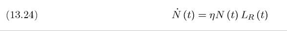
where Lr (t) is labor allocated to R&D at time t. The term N (t) on the right-hand side captures spillovers from the stock of existing ideas. The greater is N (t), the more productive is an R&D worker. Notice that (13.24) imposes that these spillovers are proportional or linear. This linearity will be the source of endogenous growth in the current model. In the next section, we will see that a different kind of endogenous growth model can be formulated with less than proportional spillovers.
In (13.24), Lr (t) is research employment, which comes out of the regular labor force. An alternative, which was originally used by Romer (1990), would be to suppose that only skilled workers or scientists can work in the knowledge-production (R&D) sector. Here we use the assumption that a homogeneous workforce is employed both in the R&D sector and in the final good sector. The advantage of this formulation is that competition between the production and the R&D sectors for workers ensures that the cost of workers to the research sector is given by the wage rate in final good sector. The only other change we need to make to the underlying environment is that now the total labor input employed in the final good sector, represented by the production function (13.2), is Le (t) rather than L, since some of 486
the workers are working in the R&D sector. Labor market clearing then requires that
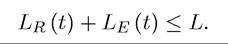
The fact that not all workers are in the final good sector implies that the aggregate output of the economy (by an argument similar to before) is given by

and profits of monopolists from selling their machines is

The net present discounted value of a monopolist (for a blueprint ν) is still given by V (ν,t) as in (13.7) or (13.8), with the flow profits given by (13.26). However, the free entry condition is no longer the same as that which followed from equation (13.4).
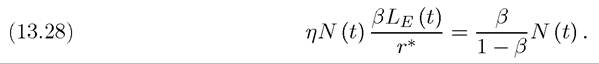
Instead, (13.24) implies the following free entry condition (when there is positive research):
where N (t) is on the left-hand side because it parameterizes the productivity of an R&D worker, while the flow cost of undertaking research is hiring workers for R&D, thus is equal to the wage rate w (t).
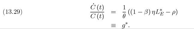
The equilibrium wage rate must be the same as in the lab equipment model of the previous section, in particular, as in equation (13.13), since the final good sector is unchanged. Thus, we still have w (t) = βN (t) / (1 — β). Moreover, balanced growth again requires that the interest rate must be constant at some level r*. Using these observations together with the free entry condition, we obtain:
Hence the BGP equilibrium interest rate must be
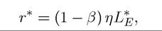
where is the number of workers employed in production in BGP (given by
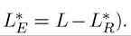 The fact that the number of workers in production must be constant in BGP follows from (13.28). Now using the Euler equation of the representative household, (13.16), we have that for all t,
To complete the characterization of the BGP equilibrium, we need to determine In
In

487
the rate of technological progress, thus g* = NI (t) /N (t). This implies that the BGP level of employment is uniquely pinned down as

The rest of the analysis is unchanged.
It can also be verified that there are no transitional dynamics in the decentralized equilibrium (see Exercise 13.17). It is also useful to note that there is again a scale effect here—greater L increases the interest rate and the growth rate in the economy.PROPOSITION 13.4. Consider the above-described expanding input-variety model with knowledge spillovers and suppose that

where is the number of workers employed in production in BGP, given by (13.30).Then there exists a unique balanced growth path in which technology, output and consumption grow at the same rate,
 given by (13.29) starting from any initial level of technology stock N (0) > 0.
Proof. Most of the proof is given by the preceding discussion. Exercise 13.16 asks you to verify that the transversality condition is satisfied and that there are no transitional dynamics. ?
Also, as in the lab equipment model, the equilibrium allocation is Pareto suboptimal, and the Pareto optimal allocation involves a higher rate of output and consumption growth. Intuitively, while firms disregard the future increases in the productivity of R&D resulting from their own R&D spending, the social planner internalizes this effect (see Exercise 13.17).
13.3.
More on the topic Growth with Knowledge Spillovers:
- THE INTERNET, ICT AND PRODUCTIVITY
- Most people think of international organizations in general as parts of an effort to prevent international war.
- Ocean currents are driven by surface winds
- CONCLUSION
- CREATIVE DESTRUCTION
- INTRODUCTION
- NETWORK EFFECTS AND ICT EXTERNALITIES
- Introduction
- Empirical studies of the effects of social capital
- Tackling the fallout from COVID-19