The AK Model Revisited

Let us start with the simplest neoclassical model of sustained growth, which we already encountered in the context of the Solow growth model, in particular, Proposition 2.10 in subsection 2.5.1.

11.1.1. Demographics, Preferences and Technology. Our focus in this chapter and the next part of the book is on economic growth, and as a first pass, we will focus on balanced economic growth, defined as a growth path consistent with the Kaldor facts (recall Chapter 2). As demonstrated in Chapter 8, balanced growth forces us to adopt the standard CRRA preferences as in the canonical neoclassical growth model (to ensure a constant intertemporal elasticity of substitution).

Throughout this chapter, we assume that the economy admits an infinitely-lived repre­sentative household, with household size growing at the exponential rate n. The preferences of the representative household at time t = 0 are given by

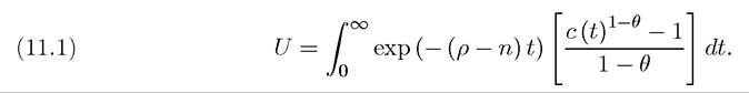
Labor is supplied inelastically. The flow budget constraint facing the household can be written

as

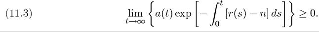
where a (t) denotes assets per capita at time t, r (t) is the interest rate, w (t) is the wage rate per capita, and n is the growth rate of population. As usual, we also need to impose the no-Ponzi game constraint:

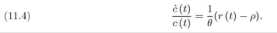
The Euler equation for the representative household is the same as before and implies the following rate of consumption growth per capita:

The other necessary condition for optimality of the consumer’s plans is the transversality condition,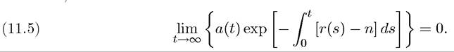

As before, the problem of the consumer is concave, thus any solution to these necessary conditions is in fact an optimal plan.

The final good sector is similar to before, except that Assumptions 1 and 2 are not satisfied. More specifically, we adopt the following aggregate production function:

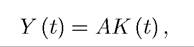
with A > 0. Notice that this production function does not depend on labor, thus wage earnings, w (t), in (11.2) will be equal to zero. This is one of the unattractive features of the baseline AK model, but will be relaxed below (and it is also relaxed in Exercises 11.3 and 11.4). Dividing both sides of this equation by L (t), and as usual, defining k (t) ? K (t) /L (t) as the capital-labor ratio, we obtain per capita output as

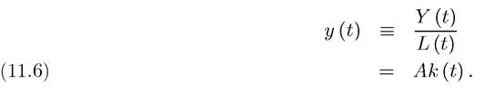
Equation (11.6) has a number of notable differences from our standard production function satisfying Assumptions 1 and 2. First, output is only a function of capital, and there are no diminishing returns (i.e., it is no longer the case that f" (∙) < 0). We will see that this feature is only for simplicity and introducing diminishing returns to capital does not affect the main results in this section (see Exercise 11.4). The more important assumption is that the Inada conditions embedded in Assumption 2 are no longer satisfied. In particular,

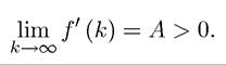
This feature is essential for sustained growth.

The conditions for profit-maximization are similar to before, and require that the marginal product of capital be equal to the rental price of capital, R (t) = r (t) + δ. Since, as is obvious from equation (11.6), the marginal product of capital is constant and equal to A, thus R (t) = A for all t, which implies that the net rate of return on the savings is constant and equal to:

Since the marginal product of labor is zero, the wage rate, w (t), is zero as noted above.

11.1.2. Equilibrium. A competitive equilibrium of this economy consists of paths of per capita consumption, capital-labor ratio, wage rates and rental rates of capital, such that the representative household maximizes (11.1) subject to (11.2) and (11.3) given initial capital-labor ratio k (0) and factor prices 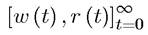such that w (t) = 0 for all t, and r (t) is given by (11.7).

To characterize the equilibrium, we again note that a (t) = k (t). Next using the fact that r = A — δ and w = 0, equations (11.2), (11.4), and (11.5) imply

The important result immediately follows from equation (11.9). Since the right-hand side of this equation is constant, there must be a constant rate of consumption growth (as long as A — δ — p > 0). The rate of growth of consumption is therefore independent of the level of capital stock per person, k (t). This will also imply that there are no transitional dynamics in this model. Starting from any k (0), consumption per capita (and as we will see, the capital-labor ratio) will immediately start growing at a constant rate. To develop this point, let us integrate equation (11.9) starting from some initial level of consumption c(0), which as usual is still to be determined later (from the lifetime budget constraint). This gives

Since there is growth in this economy, we have to ensure that the transversality condition is satisfied (i.e., that lifetime utility is bounded away from infinity), and also we want to ensure positive growth (the condition A — δ — p > 0 mentioned above). We therefore impose:

The first part of this condition ensures that there will be positive consumption growth, while the second part is the analog to the condition that ρ + θg > g + n in the neoclassical growth model with technological progress, which was imposed to ensure bounded utility (and thus was used in proving that the transversality condition was satisfied).

11.1.3. Equilibrium Characterization. We first establish that there are no transi­tional dynamics in this economy. In particular, we will show that not only the growth rate of consumption, but the growth rates of capital and output are also constant at all points in time, and equal the growth rate of consumption given in equation (11.9).

To do this, let us substitute for c(t) from equation (11.11) into equation (11.8), which

yields

which is a first-order, non-autonomous linear differential equation in k (t).

This type of

equation can be solved easily. In particular recall that if

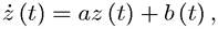
then, the solution is

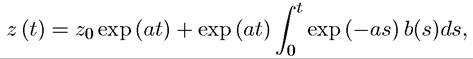
for some constant z_o chosen to satisfy the boundary conditions. Therefore, equation (11.13)

solves for:

From (11.14), it may look like capital is not growing at a constant rate, since it is the sum of two components growing at different rates. However, this is where the transversality condition becomes useful. Let us substitute from (11.14) into the transversality condition, (11.10), which yields where the second line immediately follows from the fact that the boundary condition has to hold for capital at t = 0. This equation naturally implies that capital and output grow at the same rate as consumption.

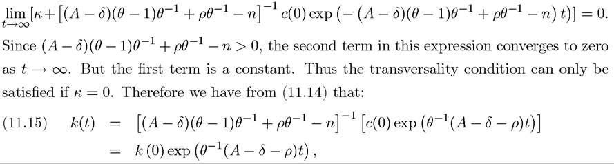
It also pins down the initial level of consumption as

Note also that in this simple AK model, growth is not only sustained, but it is also endogenous in the sense of being affected by underlying parameters.

level of income per capita—it could have no effect on the growth rate, which was determined by the exogenous labor-augmenting rate of technological progress. Here, is straightforward to verify that an increase in the discount rate, ρ, will reduce the growth rate, because it will make consumers less patient and will therefore reduce the rate of capital accumulation. Since capital accumulation is the engine of growth, the equilibrium rate of growth will decline. Similarly, changes in A and θ affect the levels and growth rates of consumption, capital and

output.

Finally, we can calculate the saving rate in this economy. It is defined as total invest­ment (which is equal to increase in capital plus replacement investment) divided by output. Consequently, the saving rate is constant and given by

where the last equality exploited the fact that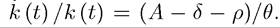This equation

implies that the saving rate, which was taken as constant and exogenous in the basic Solow model, is again constant, but is now a function of parameters, and more specifically of exactly the same parameters that determine the equilibrium growth rate of the economy.

Summarizing, we have:

Proposition 11.1. Consider the above-described AK economy, with a representative household with preferences given by (11.1), and the production technology given by (11.6). Suppose that condition (11.12) holds. Then, there exists a unique equilibrium path in which consumption, capital and output all grow at the same rate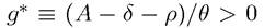starting

from any initial positive capital stock per worker k (0), and the saving rate is endogenously determined by (11.17).

One important implication of the AK model is that since all markets are competitive, there is a representative household, and there are no externalities, the competitive equilibrium will be Pareto optimal. This can be proved either using First Welfare Theorem type reasoning, or by directly constructing the optimal growth solution.

Proposition 11.2. Consider the above-described AK economy, with a representative household with preferences given by (11.1), and the production technology given by (11.6). Suppose that condition (11.12) holds. Then, the unique competitive equilibrium is Pareto optimal.

Proof. See Exercise 11.2

?

11.1.4. The Role of Policy. It is straightforward to incorporate policy differences in to this framework and investigate their implications on the equilibrium growth rate. The simplest and arguably one of the most relevant classes of policies are, as also discussed above, those affecting the rate of return to accumulation. In particular, suppose that there is an effective tax rate of τ on the rate of return from capital income, so that the flow budget constraint of the representative household becomes:

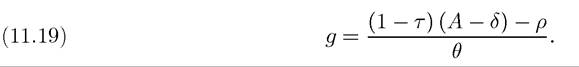
Repeating the analysis above immediately implies that this will adversely affect the growth rate of the economy, which will now become (see Exercise 11.5):

Moreover, it can be calculated that the saving rate will now be

which is a decreasing function of τ if A — δ > 0. Therefore, in this model, the equilibrium saving rate is constant as in the basic Solow model, but in contrast to that model, it responds endogenously to policy. In addition, the fact that the saving rate is constant implies that differences in policies will lead to permanent differences in the rate of capital accumulation. This observation has a very important implication. While in the baseline neoclassical growth model, even reasonably large differences in distortions (for example, eightfold differences in τ) could only have limited effects on differences in income per capita, here even small differences in τ can have very large effects. In particular, consider two economies, with respective (constant) tax rates on capital income τ and τ⁰ > τ, and exactly the same technology and preferences otherwise. It is straightforward to verify that for any τ⁰ > τ,

where Y (τ, t) denotes aggregate output in the economy with tax τ at time t. Therefore, even small policy differences can have very large effects in the long run. So why does the literature focus on the inability of the standard neoclassical growth model to generate large differences rather than the possibility that the AK model can generate arbitrarily large differences? The reason is twofold: first, for the reasons already discussed, the AK model, with no diminishing returns and the share of capital in national income asymptoting to 1, is not viewed as a good approximation to reality. Second, and related to our discussion in Chapter 1, most economists believe that the relative stability of the world income distribution in the post-war era makes it more attractive to focus on models in which there is a stationary world income distribution, rather than models in which small policy differences can lead to permanent growth differences. Whether this last belief is justified is, in part, an empirical question.

11.2.