The AK Model with Physical and Human Capital

As pointed out in the previous section, a major shortcoming of the baseline AK model is that the share of capital accruing to national income is equal to 1 (or limits to 1 as in the variant of the AK model studied in Exercises 11.3 and 11.4).

where H (t) denotes efficiency units of labor (or human capital), which will be accumulated in the same way as physical capital. We assume that the production function F (∙, ∙) now satisfies our standard assumptions, Assumptions 1 and 2.

Suppose that the budget constraint of the representative household is given by where h (t) denotes the effective units of labor (human capital) on the representative house­hold, w (t) is wage rate per unit of human capital, and ⅛ (t) is investment in human capital. The human capital of the representative household evolves according to the differential equa­tion:

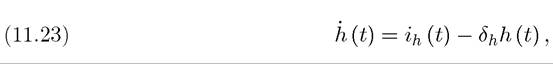
where δh is the depreciation rate of human capital. The evolution of the capital stock is again given from the observation that k (t) = a (t), and we now denote the depreciation rate of physical capital by δ_k to avoid confusion with δ⅛. In this model, the representative household maximizes its utility by choosing the paths of consumption, human capital investments and asset holdings.

where, now, the effective capital-labor ratio is given by dividing the capital stock by the stock of human capital in the economy,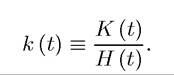

A competitive equilibrium of this economy consists of paths of per capita consumption, capital-labor ratio, wage rates and rental rates of capital,such

that the representative household maximizes (11.1) subject to (11.3), (11.22) and (11.23) given initial effective capital-labor ratio k (0) and factor pricesthat satisfy

(11.24).

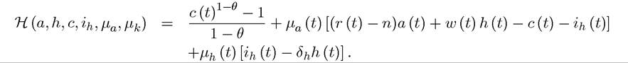
To characterize the competitive equilibrium, let us first set up at the current-value Hamil­tonian for the representative household with costate variables μ_a and μ_h:

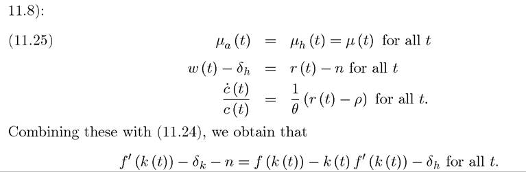
Now the necessary conditions of this optimization problem imply the following (see Exercise

Since the left-hand side is decreasing in k (t), while the right-hand side is increasing, this implies that the effective capital-labor ratio must satisfy

k (t) = k* for all t.

We can then prove the following proposition:

Proposition 11.3. Consider the above-described AK economy with physical and human capital, with a representative household with preferences given by (11.1), and the production technology given by (11.21). Let k* be given by

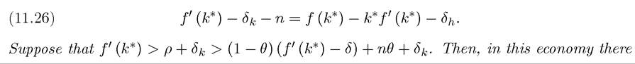
exists a unique equilibrium path in which consumption, capital and output all grow at the same rate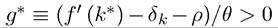starting from any initial conditions, where k* is given

by (11.26).The share of capital in national income is constant at all times.

Proof. See Exercise 11.9 ?

The advantage of the economy studied here, especially as compared to the baseline AK model is that, it generates a stable factor distribution of income, with a significant fraction of national income accruing to labor as rewards to human capital. Consequently, the current model cannot be criticized on the basis of generating counter-factual results on the capital share of GDP. A similar analysis to that in the previous section also shows that the current model generates long-run growth rate differences from small policy differences. Therefore, it can account for arbitrarily large differences in income per capita across countries. Neverthe­less, it would do so partly by generating large human capital differences across countries. As 425

such, the empirical mechanism through which these large cross-country income differences are generated may again not fit with the empirical patterns discussed in Chapter 3. More­over, given substantial differences in policies across economies in the postwar period, like the baseline AK economy, the current model would suggest significant changes in the world income distribution, whereas the evidence in Chapter 1 points to a relatively stable postwar world income distribution.

11.3.