The Two-Sector AK Model

The models studied in the previous two sections are attractive in many respects; they generate sustained growth, and the equilibrium growth rate responds to policy, to underlying preferences and to technology.

One unattractive feature of the baseline AK model is that all of national income accrues to capital. Essentially, it is a one-sector model with only capital as the factor of production. This makes it difficult to apply this model to real world situations. The model in the previous section avoids this problem, but at some level it does so by creating another factor of pro­duction that accumulates linearly, so that the equilibrium structure is again equivalent to the one-sector AK economy. Therefore, in some deep sense, the economies of both sections are one-sector models. More important than this one-sector property, these models potentially blur key underlying characteristic driving growth in these environments. What is important is not that the production technology is AK, but the related feature that the accumulation technology is linear. In this section, we will discuss a richer two-sector model of neoclassical endogenous growth, based on Rebelo’s (1991) work. This model will generate constant factor shares in national income without introducing human capital accumulation. Perhaps more importantly, it will illustrate the role of differences in the capital intensity of the production functions of consumption and investment.

The preference and demographics are the same as in the model of the previous section, in particular, equations (11.1)-(11.5) apply as before (but with a slightly different interpretation for the interest rate in (11.4) as will be discussed below). Moreover, to simplify the analysis, suppose that there is no population growth, i.e., n = O, and that the total amount of labor in the economy, L, is supplied inelastically.

The main difference is in the production technology. Rather than a single good used for consumption and investment, we now envisage an economy with two sectors. Sector 1 produces consumption goods with the following technology

where the subscript “C” denotes that these are capital and labor used in the consumption sector, which has a Cobb-Douglas technology. In fact, the Cobb-Douglas assumption here is quite important in ensuring that the share of capital in national income is constant (see Exercise 11.12). The capital accumulation equation is given by:

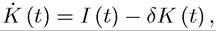
where I (t) denotes investment. Investment goods are produced with a different technology than (11.27), however. In particular, we have

The distinctive feature of the technology for the investment goods sector, (11.28), is that it is linear in the capital stock and does not feature labor. This is an extreme version of an assumption often made in two-sector models, that the investment-good sector is more capital-intensive than the consumption-good sector. In the data, there seems to be some support for this, though the capital intensities of many sectors have been changing over time as the nature of consumption and investment goods has changed.

Market clearing implies:

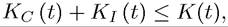
for capital, and

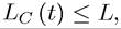
for labor (since labor is only used in the consumption sector).

An equilibrium in this economy is defined similarly to that in the neoclassical economy, but also features an allocation decision of capital between the two sectors. Moreover, since the two sectors are producing two different goods, consumption and investment goods, there will be a relative price between the two sectors which will adjust endogenously.

Since both market clearing conditions will hold as equalities (the marginal product of both factors is always positive), we can simplify notation by letting κ (t) denote the share of capital used in the investment sector

From profit maximization, the rate of return to capital has to be the same when it is employed in the two sectors. Let the price of the investment good be denoted by pi (t) and that of the consumption good by pc (t), then we have

Define a steady-state (a balanced growth path) as an equilibrium path in which κ (t) is

constant and equal to some κ ∈ [0,1]. Moreover, let us choose the consumption good as the 427

numeraire, so that pc (t) = 1 for all t. Then differentiating (11.29) implies that at the steady state:

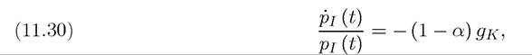
where gκ is the steady-state (BGP) growth rate of capital.

As noted above, the Euler equation for consumers, (11.4), still holds, but the relevant interest rate has to be for consumption-denominated loans, denoted by rc (t). In other words, it is the interest rate that measures how many units of consumption good an individual will receive tomorrow by giving up one unit of consumption today. Since the relative price of consumption goods and investment goods is changing over time, the proper calculation goes as follows. By giving up one unit of consumption, the individual will buy 1/pi (t) units of capital goods. This will have an instantaneous return of rj (t). In addition, the individual will get back the one unit of capital, which has now experienced a change in its price of and finally, he will have to buy consumption goods, whose prices changed by.

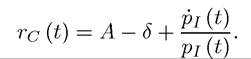
Therefore, the general formula of the rate of return denominated in consumption goods in terms of the rate of return denominated in investment goods is

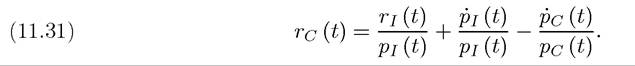
In our setting, given our choice of numeraire, we haveMoreover,

is given by (11.30). Finally,

given the linear technology in (11.28). Therefore, we have

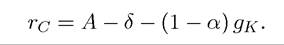
and in steady state, from (11.30), the steady-state consumption-denominated rate of return is:

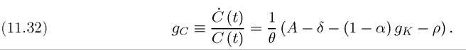
From (11.4), this implies a consumption growth rate of

Finally, differentiate (11.27) and use the fact that labor is always constant to obtain 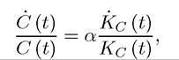which, from the constancy of κ(t) in steady state, implies the following steady-state relation­ship:

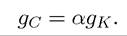
428

Substituting this into (11.32), we have

and

What about wages? Because labor is being used in the consumption good sector, there will be positive wages. Since labor markets are competitive, the wage rate at time t is given by

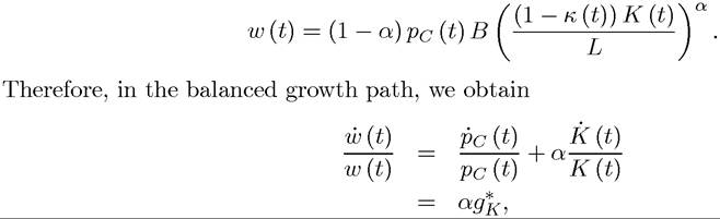
which implies that wages also grow at the same rate as consumption.

Moreover, with exactly the same arguments as in the previous section, it can be estab­lished that there are no transitional dynamics in this economy. This establishes the following result:

Proposition 11.4. In the above-described two-sector neoclassical economy, starting from any K (0) > 0, consumption and labor income grow at the constant rate given by (11.34), while the capital stock grows at the constant rate (11.33).

It is straightforward to conduct policy analysis in this model, and as in the basic AK model, taxes on investment income will depress growth. Similarly, a lower discount rate will increase the equilibrium growth rate of the economy

One important implication of this model, different from the neoclassical growth model, is that there is continuous capital deepening. Capital grows at a faster rate than consumption and output. Whether this is a realistic feature is debatable. The Kaldor facts, discussed above, include constant capital-output ratio as one of the requirements of balanced growth. Here we have steady state and “balanced growth” without this feature. For much of the 20th century, capital-output ratio has been constant, but it has been increasing steadily over the past 30 years. Part of the reason why it has been increasing recently but not before is because of relative price adjustments. New capital goods are of higher quality, and this needs to be incorporated in calculating the capital-output ratio. These calculations have only been performed in the recent past, which may explain why capital-output ratio has been constant in the earlier part of the century, but not recently.

11.4.