The Real Business Cycle Theory

Summarize the real business cycle theory and describe how well it accounts for the business cycle facts.

We have identified two basic questions of business cycle analysis: What causes business cycles? and What can (or should) be done about them? Let's examine the classical answers to these questions, beginning with what causes business cycles.

Recall from Section 8.4 that a complete theory of the business cycle must have two components. The first is a description of the types of shocks or disturbances believed to affect the economy the most. Examples of economic disturbances emphasized by various theories of the business cycle include supply shocks, changes in monetary or fiscal policy, and changes in consumer spending. The second compo­nent is a model that describes how key macroeconomic variables, such as output, employment, and prices, respond to economic shocks. Classical economists prefer to build their models from microeconomic foundations, describing how people maximize their utility and how firms maximize profits. Thus their preferred models are quite complex and we cannot represent them easily in this textbook. However, the main results of their detailed models are similar to those from the market-clearing version of the IS-LM model, so in this text we will use that model to represent the views of classical macroeconomists. In addition, the issue of which shocks are crucial in driving cyclical fluctuations remains.

An influential group of classical macroeconomists, led by Nobel laureates Edward Prescott of Arizona State University and the Federal Reserve Bank of Minneapolis and Finn Kydland of the University of California at Santa Barbara, developed a theory that takes a strong stand on the sources of shocks that cause cyclical fluctuations. This theory, the real business cycle theory (or RBC theory), argues that real shocks to the economy are the primary cause of business cycles.^[163] Real shocks are disturbances to the "real side" of the economy, such as shocks that affect the production function, the size of the labor force, the real quantity of government purchases, and the spending and saving decisions of consumers.

Although many types of real shocks could contribute to the business cycle, RBC economists give the largest role to production function shocks—what we've called supply shocks and what the RBC economists usually refer to as productivity shocks. Productivity shocks include the development of new products or production meth­ods, the introduction of new management techniques, changes in the quality of cap­ital or labor, changes in the availability of raw materials or energy, unusually good or unusually bad weather, changes in government regulations affecting production, and any other factor affecting productivity. According to RBC economists, most eco­nomic booms result from beneficial productivity shocks, and most recessions are caused by adverse productivity shocks.

The Recessionary Impact of an Adverse Productivity Shock. Does the RBC econo­mists' idea that adverse productivity shocks lead to recessions (and, similarly, that beneficial productivity shocks lead to booms) make sense? We examined the theoreti­cal effects on the economy of a temporary adverse productivity shock in Chapters 3, 8, and 9.^[164] In Chapter 3 we showed that an adverse productivity shock (or supply shock), such as an increase in the price of oil, reduces the marginal product of labor (MPN) and the demand for labor at any real wage. As a result, the equilibrium values of the real wage and employment both fall (see Fig. 3.10). The equilibrium level of output (the full-employment level of output Y) also falls, both because equilibrium employ­ment declines and because the adverse productivity shock reduces the amount of out­put that can be produced by any amount of capital and labor.

We later used the complete IS-LM model (Fig. 9.8) to explore the general equi­librium effects of a temporary adverse productivity shock.

Broadly, then, our earlier analyses of the effects of an adverse productivity shock support the RBC economists' claim that such shocks are recessionary, in that they lead to declines in output. Similar analyses show that a beneficial productivity shock leads to a rise in output (a boom). Note that, in the RBC approach, output declines in recessions and rises in booms because the general equilibrium (or full-employment) level of output has changed and because rapid price adjustment ensures that actual output always equals full-employment output. As classical economists, RBC econo­mists would reject the Keynesian view (which we will discuss in Chapter 11) that recessions and booms are periods of disequilibrium, during which actual output is below or above its general equilibrium level for a protracted period of time.

Real Business Cycle Theory and the Business Cycle Facts. Although the RBC theory—which combines the classical, or market-clearing, version of the IS-LM model with the assumption that productivity shocks are the dominant form of eco­nomic disturbance—is relatively simple, it is consistent with many of the basic busi­ness cycle facts. First, under the assumption that the economy is being continuously buffeted by productivity shocks, the RBC approach predicts recurrent fluctuations in aggregate output, which actually occur. Second, the RBC theory correctly predicts that employment will move procyclically—that is, in the same direction as output. Third, the RBC theory predicts that real wages will be higher during booms than during recessions (procyclical real wages), as also occurs.

A fourth business cycle fact explained by the RBC theory is that average labor productivity is procyclical; that is, output per worker is higher during booms than during recessions.

A business cycle fact that does not seem to be consistent with the simple RBC theory is that inflation tends to slow during or immediately after a recession. The theory predicts that an adverse productivity shock will both cause a recession and increase the general price level. Thus according to the RBC approach, periods of recession should also be periods of inflation, contrary to the business cycle fact.

Some RBC economists have responded by taking issue with the conventional view that inflation is procyclical. For example, in a study of the period 1954-1989, RBC proponents Kydland and Prescott^[165] showed that the finding of procyclical inflation is somewhat sensitive to the statistical methods used to calculate the trends in inflation and output. Using a different method of calculating these trends, Kydland and Prescott found evidence that, when aggregate output has been above its long-run trend, the price level has tended to be below its long-run trend, a result more nearly consistent with the RBC prediction about the cyclical behavior of prices.

Application

Calibrating the Business Cycle

If we put aside the debate about price level behavior, the RBC theory can account for some of the business cycle facts, including the procyclical behavior of employ­ment, productivity, and real wages. However, real business cycle economists argue that an adequate theory of the business cycle should be quantitative as well as quali­tative. In other words, in addition to predicting generally how key macroeconomic variables move throughout the business cycle, the theory should predict numeri­cally the size of economic fluctuations and the strength of relationships among the variables.

To examine the quantitative implications of their theories, RBC economists developed a method called calibration. The idea is to work out a detailed numeri­cal example of a more general theory. The results are then compared to macroeco­nomic data to see whether model and reality broadly agree.

The first step in calibration is to write down a model of the economy—such as the classical version of the IS-LM model—except that specific functions replace general functions. For example, instead of representing the production function in general terms as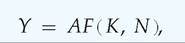

the person doing the calibration uses a specific algebraic form for the production function, such as⁴

where a is a number between 0 and 1. Similarly, specific functions are used to describe the behavior of consumers and workers.

Next, the specific functions chosen are made even more specific by expressing them in numerical terms. For example, for a = 0.3, the production function becomes

In the same way, specific numbers are assigned to the functions describing the behavior of consumers and workers. Where do these numbers come from? Generally, they are not estimated from macroeconomic data but are based on other sources.

For example, the numbers assigned to the functions in the model may come from previous studies of the production function or of the saving behavior of individuals and families.

⁴This production function is the Cobb-Douglas production function (Chapter 3). As we noted,

although it is relatively simple, it fits U.S. data quite well.

(continued)

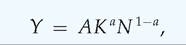
FIGURE 10.1

Actual versus simulated volatilities of key macroeconomic variables

The figure compares the actual volatilities of key macroeconomic variables observed in post-World War II U.S. data with the volatilities of the same variables predicted by computer simulations of Edward Prescott's calibrated RBC model. Prescott set the size of the random productivity shocks in his simulations so that the simulated volatility of GNP would match the actually observed volatility of GNP exactly. For these random productivity shocks, the simulated volatilities of the other five macroeconomic variables (with the possible exception of consumption) match the observed volatilities fairly well.

The third step, which must be carried out on a computer, is to find out how the numerically specified model behaves when it is hit by random shocks, such as pro­ductivity shocks. The shocks are created on the computer with a random number generator, with the size and persistence of the shocks (unlike the numbers assigned to the specific functions) being chosen to fit the actual macroeconomic data. For these shocks, the computer tracks the behavior of the model over many periods and reports the implied behavior of key macroeconomic variables such as output, employment, consumption, and investment. The results from these simulations are then compared to the behavior of the actual economy to determine how well the model fits reality.

Edward Prescott^[166] performed an early and influential calibration exercise. He used a model similar to the RBC model we present here, the main difference being that our version of the RBC model is essentially a two-period model (the present and the future), and Prescott's model allowed for many periods. The results of his computer simulations are shown in Figures 10.1 and 10.2.

Figure 10.1 compares the actually observed volatilities of six macroeconomic variables, as calculated from post-World War II U.S. data, with the volatilities pre­dicted by Prescott's calibrated RBC model.^[167] Prescott set the size of the random productivity shocks in his simulations so that the volatility of GNP in his model would match the actual volatility in U.S. GNP.^[168] That choice explains why the

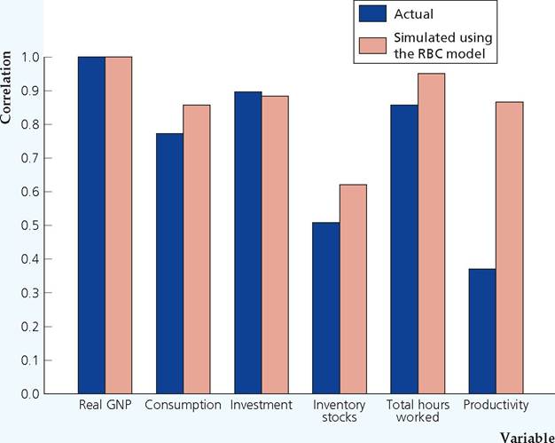
FIGUREJ0.2

Actual versus simulated correlations of key macroeconomic variables with GNP How closely a variable moves with GNP over the business cycle is measured by its correlation with GNP, with higher correlations implying a closer relationship. The figure compares the correlations of key variables with GNP that were actually observed in the post-World War II U.S. economy with the correlations predicted by computer simulations of Prescott's calibrated RBC model. Except for productivity, whose predicted correlation with GNP is too high, the simulations predicted correlations of macroeconomic variables with GNP that closely resemble the actual correlations of these variables with GNP.

actual and simulated volatilities of GNP are equal in Fig. 10.1. But he did nothing to guarantee that the simulation would match the actual volatilities of the other five variables. Note, however, that the simulated and actual volatilities for the other variables in most cases are quite close.

Figure 10.2 compares the actual economy with Prescott's calibrated model in another respect: how closely important macroeconomic variables move with GNP over the business cycle. The statistical measure of how closely variables move together is called correlation. If a variable's correlation with GNP is posi­tive, the variable tends to move in the same direction as GNP over the busi­ness cycle (that is, the variable is procyclical). A correlation with GNP of 1.0 indicates that the variable's movements track the movements of GNP perfectly (thus the correlation of GNP with itself is 1.0), and a correlation with GNP of 0 indicates no relationship to GNP. Correlations with GNP between 0 and 1.0 reflect relationships with GNP of intermediate strength. Figure 10.2 shows that Prescott's model generally accounts well for the strength of the relationships between some of the variables and GNP, although the correlation of productiv­ity and GNP predicted by Prescott's model is noticeably larger than the actual correlation.

The degree to which relatively simple calibrated RBC models can match the actual data is impressive. In addition, the results of calibration exercises help guide further development of the model. For example, the version of the RBC model discussed here has been modified to improve the match between the actual and predicted correlations of productivity with GNP.

Are Productivity Shocks the Only Source of Recessions? Although RBC economists agree in principle that many types of real shocks buffet the economy, in practice much of their work rests on the assumption that productivity shocks are the dominant, or even the only, source of recessions. Many economists, including both classicals and Keynesians, have criticized this assumption as being unrealistic. For example, some economists challenged the RBC economists to identify the specific productivity shocks that they believe caused each of the recessions since World War II. The critics argue that, except for the oil price shocks of 1973, 1979, and 1990, and the tech revolution of the late 1990s, historical exam­ples of economywide productivity shocks are virtually nonexistent.

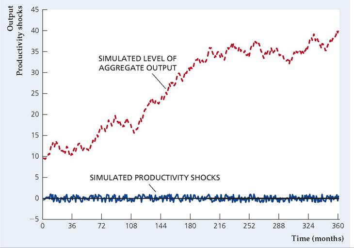
An interesting RBC response to that argument is that, in principle, economy­wide fluctuations could also be caused by the cumulative effects of a series of small productivity shocks. To illustrate the point that small shocks can cause large fluctua­tions, Figure 10.3 shows the results of a computer simulation of productivity shocks and the associated behavior of output for a simplified RBC model. In this simple RBC model, the change in output from one month to the next has two parts: (1) A fixed part that arises from normal technical progress or from a normal increase in population and employment and (2) an unpredictable part that reflects a random shock to productivity during the current month.^[169] The random, computer-generated productivity shocks are shown at the bottom of Fig. 10.3, and the implied behavior of output is displayed above them. Although none of the individual shocks is large, the cumulative effect of the shocks causes large fluctuations in output that look something like business cycles. Hence business cycles may be the result of produc­tivity shocks, even though identifying specific, large shocks is difficult.

Does the Solow Residual Measure Technology Shocks? Because productivity shocks are the primary source of business cycle fluctuations in RBC models, RBC economists have attempted to measure the size of these shocks. The most common measure of productivity shocks is known as the Solow residual, which is an empiri­cal measure of total factor productivity, A. The Solow residual is named after the orig­inator of modern growth theory, Robert Solow,^[170] who used this measure in the 1950s.

Recall from Chapter 3 that, to measure total factor productivity A, we need data on output, Y, and the inputs of capital, K, and labor, N. In addition, we need to use a specific algebraic form for the production function. Then we have

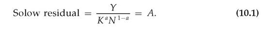
The Solow residual is called a "residual" because it is the part of output that cannot be directly explained by measured capital and labor inputs.

When the Solow residual is computed from actual U.S. data, using Eq. (10.1), it turns out to be strongly procyclical, rising in economic expansions and falling in recessions. This procyclical behavior is consistent with the premise of RBC theory that cyclical fluctuations in aggregate output are driven largely by productivity shocks.

FIGUREJ0.3

Small shocks and large cycles

A computer simulation of a simple RBC model is used to find the relation­ship between computer­generated random productivity shocks (shown at the bottom of the figure) and aggregate output (shown in the middle of the figure). Even though all of the productivity shocks are small, the simulation produces large cyclical fluctuations in aggregate output. Thus large productivity shocks aren't necessary to generate large cyclical fluctuations.

However, some economists have questioned whether the Solow residual should be interpreted solely as a measure of technology, as early RBC proponents tended to do. If changes in the Solow residual reflect only changes in the technolo­gies available to an economy, its value should be unrelated to factors such as government purchases or monetary policy that don't directly affect scientific and technological progress (at least in the short run). However, statistical studies reveal that the Solow residual is in fact correlated with factors such as government expenditures, suggesting that movements in the Solow residual may also reflect the impacts of other factors.^[171]

To understand why measured productivity can vary, even if the actual tech­nology used in production doesn't change, we need to recognize that capital and labor sometimes are used more intensively than at other times and that more intensive use of inputs leads to higher output. For instance, a robotic car assembly tool used full-time contributes more to production than an otherwise identical tool used half-time. Similarly, workers working rapidly (for example, restaurant work­ers during a busy lunch hour) will produce more output and revenue than the same number of workers working more slowly (the same restaurant workers dur­ing the afternoon lull). To capture the idea that capital and labor resources can be used more or less intensively at different times, we define the utilization rate of capi­tal, u_κ, and the utilization rate of labor, u_N. The utilization rate of a factor measures the intensity at which it is being used. For example, the utilization rate of capital for the printing press run full-time would be twice as high as for the printing press

used half-time; similarly, the utilization rate of labor is higher in the restaurant during lunch hour. The actual usage of the capital stock in production, which we call capital services, equals the utilization rate of capital times the stock of capital, or u_κK. Capital services are a more accurate measure of the contribution of the capi­tal stock to output than is the level of capital itself because the definition of capital services adjusts for the intensity at which capital is used. Similarly, we define labor services to be the utilization rate of labor times the number of workers (or hours) employed by the firm, or u_nN. Thus the labor services received by an employer are higher when the same number of workers are working rapidly than when they are working slowly (that is, the utilization of labor is higher).

Recognizing that capital services and labor services go into the production of output, we rewrite the production function as

where we have replaced the capital stock, K, with capital services, u_κK, and labor, N, with labor services, u_nN. Now we can use the production function in Eq. (10.2) to substitute for Y in Eq. (10.1) to obtain an expression for the Solow residual that incorporates utilization rates for capital and labor:

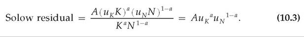
Equation (10.3) shows that the Solow residual, as conventionally measured, includes not only parameter A (which reflects technology and perhaps other factors affecting productivity) but also utilization rates of capital and labor, u_κ and u_N. Thus even if technology were unchanging, the calculated Solow residual would be procyclical if the utilization rates of capital and labor were procyclical.

There is evidence that utilization is procyclical (so that capital and labor are worked harder in boom periods than in economic slumps). For example, Craig Burnside of Duke University, and Martin Eichenbaum and Sergio Rebelo¹¹, both of Northwestern University, studied the cyclical behavior of capital utilization by using data on the amount of electricity used by producers. Their rationale for using data on electricity is that additional electricity is needed to increase capital utiliza­tion, whether the increased utilization is achieved by operating capital for an increased number of hours per day or by increasing the speed at which the capital is operated. This study revealed that electricity used per unit of capital rises in eco­nomic upturns, leading the authors to conclude that capital utilization is strongly procyclical. In addition, this study showed that a measure of technology, analogous to the term A in Eq. (10.2), is much less procyclical than is the Solow residual.

Measuring the cyclical behavior of labor utilization is more difficult, but var­ious studies have found evidence that the utilization rate of labor is also procy­clical. For example, Jon Fay and James Medoff^{[172] [173] of Harvard University sent questionnaires to large manufacturing enterprises, asking about employment and production during the most recent downturn experienced at each plant. Fay and Medoff found that during a downturn the average plant surveyed cut production by 31% and cut its total use of blue-collar hours to 23% below the normal level.}

Plant managers estimated that total hours could have been reduced by an addi­tional 6% of the normal level without further reducing output. Of this 6% of nor­mal hours, about half (3% of normal hours) were typically assigned to various types of useful work, including equipment maintenance and overhaul, painting, cleaning, reworking output, and training. The remaining 3% of normal hours were assigned to "make-work" and other unproductive activities. These numbers sug­gest that firms utilize labor less intensively during recessions.

The tendency to use workers less intensively in recessions than in expansions has been referred to as labor hoarding. Labor hoarding occurs when, because of the costs of firing and hiring workers, firms retain some workers in a recession that they would otherwise lay off. Firms keep these workers on the payroll to avoid the costs of laying off workers and then rehiring them or hiring and training new workers when the economy revives. Hoarded labor either works less hard during the recession (there is less to do) or is put to work doing tasks, such as maintaining equipment, that aren't measured as part of the firm's output. When the economy revives, the hoarded labor goes back to working in the normal way. In much the same way, it may not pay the restaurant owner to send her workers home between the lunch and dinner rush hours, with the result that restaurant workers are less productive during the slow afternoon period. This lower rate of pro­ductivity during recessions (or during the afternoon slow period, in the restaurant) doesn't reflect changes in the available technology, but only changes in the rate at which firms utilize capital and labor. Hence you should be cautious about inter­preting cyclical changes in the Solow residual (equivalently, total factor produc­tivity, A) as solely reflecting changes in technology.

Although changes in technology or the utilization rates of capital and labor might cause aggregate cyclical fluctuations, history suggests that shocks other than productivity shocks also affect the economy; wars and the corresponding military buildups are but one obvious example. Thus many classical economists favor a broader definition of classical business cycle theory that allows for both productiv­ity and other types of shocks to have an impact on the economy. Because the mod­els they use allow for shocks other than "real" productivity shocks, the models are not called RBC models but rather dynamic, stochastic, general equilibrium (DSGE) models, as they model behavior over time (dynamic), allow for shocks to the econ­omy (stochastic), and are based on general equilibrium concepts.

The macroeconomic effects of shocks other than productivity shocks can be analyzed with the classical IS-LM model. Let's use it to examine the effects of fiscal policy shocks.

10.2