The Solow Model in Discrete Time
I next present the dynamics of economic growth in the discrete-time Solow model.
2.2.1. Fundamental Law of Motion of the Solow Model. Recall that K depreciates exponentially at the rate δ, so that the law of motion of the capital stock is given by
(2.8) K (t + 1) = (1 - δ) K (t)+ I (t),
where I (t) is investment at time t.
From national income accounting for a closed economy, the total amount of final good in the economy must be either consumed or invested, thus
(2.9)
Y (t) = C (t) +1 (t),
40
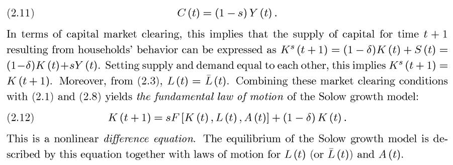
where C (t) is consumption.[2] Using (2.1), (2.8) and (2.9), any feasible dynamic allocation in this economy must satisfy

for t = 0,1,.... The question is to determine the equilibrium dynamic allocation among the set of feasible dynamic allocations. Here the behavioral rule that households save a constant fraction of their income simplifies the structure of equilibrium considerably (this is a “behavioral rule” since it is not derived from the maximization of a well-defined utility function). One implication of this assumption is that any welfare comparisons based on the Solow model have to be taken with a grain of salt, since we do not know what the preferences of the individuals are.
Since the economy is closed (and there is no government spending), aggregate investment is equal to savings,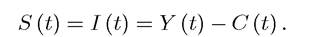
The assumption that households save a constant fraction s ∈ (0,1) of their income can be expressed as

which, in turn, implies that they consume the remaining 1 — s fraction of their income, and thus
2.2.2.
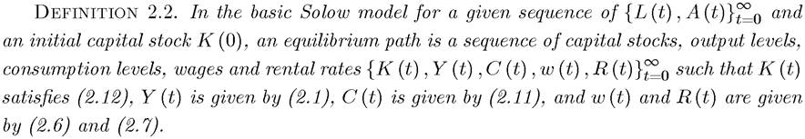
Definition of Equilibrium. The Solow model is a mixture of an old-style Keynesian model and a modern dynamic macroeconomic model. Households do not optimize when it comes to their savings/consumption decisions. Instead, their behavior is captured by eq.’s (2.10) and (2.11). Nevertheless, firms still maximize and factor markets do clear. Thus it is useful to start defining equilibria in the way that is customary in modern dynamic macro models.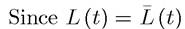 from (2.3), throughout I write the exogenous evolution of
 labor endowments in terms of L (t) to simplify notation.
The most important point to note about Definition 2.2 is that an equilibrium is defined as an entire path of allocations and prices. An economic equilibrium does not refer to a static object; it specifies the entire path of behavior of the economy.
2.2.3. Equilibrium Without Population Growth and Technological Progress.
It is useful to start with the following assumptions, which will be relaxed later in this chapter:
(1) There is no population growth; total population is constant at some level L > 0. Moreover, since individuals supply labor inelastically, this implies L (t) = L.
(2) There is no technological progress, so that A (t) = A.
Let us define the capital-labor ratio of the economy as
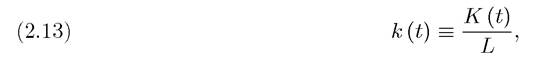
which is a key object for the analysis. Now using the constant returns to scale assumption, output (income) per capita, y (t) ? Y (t) /L, can be expressed as
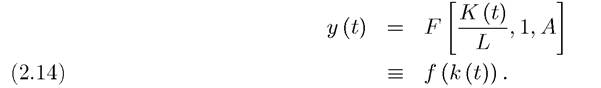
In other words, with constant returns to scale output per capita is simply a function of the capital-labor ratio. Note that f (k) here depends on A, so I could have written f (k,A).
I do not do this to simplify the notation and also because until Section 2.7, there will be no technological progress. Thus, for now A is constant and can be normalized to A = 1.3 From Theorem 2.1, the marginal products of capital and labor (and thus their rental prices) can be reexpressed as: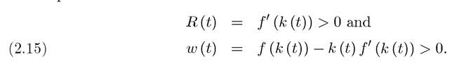
The fact that both of these factor prices are positive follows from Assumption 1, which imposed that the first derivatives of F with respect to capital and labor are always positive.
EXAMPLE 2.1. (The Cobb-Douglas Production Function) Let us consider the most common example of production function used in macroeconomics, the Cobb-Douglas production function. Let us immediately add the caveat that even though the Cobb-Douglas form is convenient and widely used, it is also very special, and many interesting phenomena
3
3Later, when technological change is taken to be “labor-augmenting,” the term A can also be taken out and the per capita production function can be written as y = Af (k), with a slightly different definition of k as effective capital-labor ratio (see, for example, equation (2.46) in Section 2.7). discussed later in this book are ruled out by this production function. The Cobb-Douglas production function can be written as
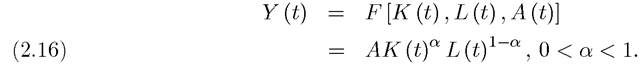
It can easily be verified that this production function satisfies Assumptions 1 and 2, including the constant returns to scale feature imposed in Assumption 1. Dividing both sides by L (t), the per capita production function in (2.14) becomes: 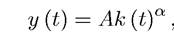
where y (t) again denotes output per worker and k (t) is capital-labor ratio as defined in (2.13). The representation of factor prices as in (2.15) can also be verified. From the per capita production function representation, in particular eq.
(2.15), the rental price of capital can be expressed as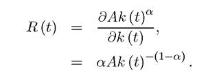
Alternatively, in terms of the original production function (2.16), the rental price of capital in (2.7) is given by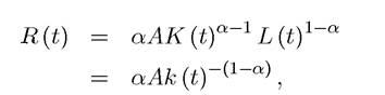
which is equal to the previous expression and thus verifies the form of the marginal product given in eq. (2.15). Similarly, from (2.15),
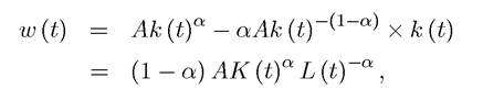
which verifies the alternative expression for the wage rate in (2.6).
Returning to the analysis with the general production function, the per capita representation of the aggregate production function enables us to divide both sides of (2.12) by L to obtain the following simple difference equation for the evolution of the capital-labor ratio:

Since this difference equation is derived from (2.12), it also can be referred to as the equilibrium difference equation of the Solow model: it describes the equilibrium behavior of the key ob ject of the model, the capital-labor ratio. The other equilibrium quantities can all be obtained from the capital-labor ratio k (t).
At this point, let us also define a steady-state equilibrium for this model.
Definition 2.3. A steady-state equilibrium without technological progress and population growth is an equilibrium path in which k (t) = k* for all t.
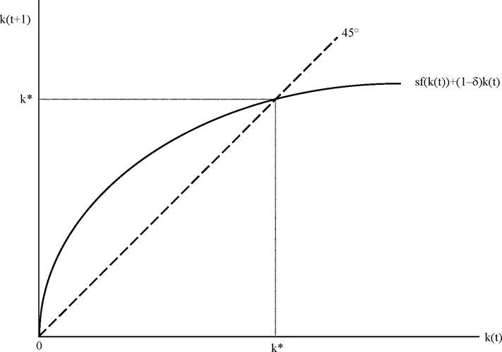
Figure 2.2. Determination of the steady-state capital-labor ratio in the Solow model without population growth and technological change.
In a steady-state equilibrium the capital-labor ratio remains constant. Since there is no
population growth, this implies that the level of the capital stock will also remain constant.
Mathematically, a “steady-state equilibrium” corresponds to a “stationary point” of the equilibrium difference equation (2.17). Most of the models in this book will admit a steady-state equilibrium and the economy will typically tend to this steady-state equilibrium over time.This is also the case for this simple model.
This can be seen by plotting the difference equation that governs the equilibrium behavior of this economy, (2.17), which is done in Figure 2.2. The thick curve represents the righthand side of eq. (2.17) and the dashed line corresponds to the 45o line. Their (positive) intersection gives the steady-state value of the capital-labor ratio k*, which satisfies

Notice that in Figure 2.2 there is another intersection between (2.17) and the 450 line at k = 0. This is because, from Assumption 2, capital is an essential input, and thus f (0) = 0. With no production, there are no savings, and the system remains at k = 0, making k = 0
a steady-state equilibrium. I will ignore this intersection throughout. This is for a number of reasons. First, k = 0 is a steady-state equilibrium only when capital is an essential input and f (0) = 0, but this assumption can be relaxed without any affect on the rest of the results. If capital were not essential, f (0) will be positive and k = 0 will cease to be a steady-state equilibrium. This is illustrated in Figure 2.3, which draws (2.17) for the case where f (0) = ε for any ε > 0. Second, as we will see below, this intersection, even when it exists, is an unstable point, thus the economy would never travel towards this point starting with K (0) > 0. Finally, and most importantly, this intersection has no economic interest for
4
us.
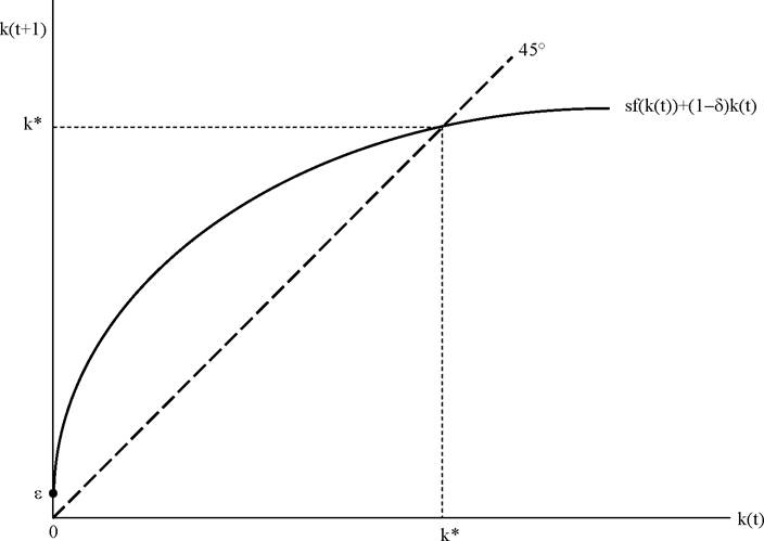
Figure 2.3. Unique steady state in the basic Solow model when f (0) = ε > 0.
An alternative visual representation shows the steady state as the intersection between a ray through the origin with slope δ (representing the function δk) and the function sf (k). Figure 2.4 illustrates this and is also useful for two other purposes. First, it depicts the levels of consumption and investment in a single figure. The vertical distance between the horizontal axis and the δk line at the steady-state equilibrium gives the amount of investment per capita at the steady-state equilibrium (equal to δk*), while the vertical distance between the function f (k) and the δk line at k* gives the level of consumption per capita. Clearly, the sum of these two terms make up f (k*). Second, Figure 2.4 also emphasizes that the steady-state equilibrium in the Solow model essentially sets investment, sf (k), equal to the amount of capital that needs to be “replenished”, δk. This interpretation will be particularly useful when population growth and technological change are incorporated.
4Hakenes and Irmen (2006) show that even with f (0) = 0, the Inada conditions imply that in the continuous-time version of the Solow model k = 0 may not be a steady-state equilibrium.
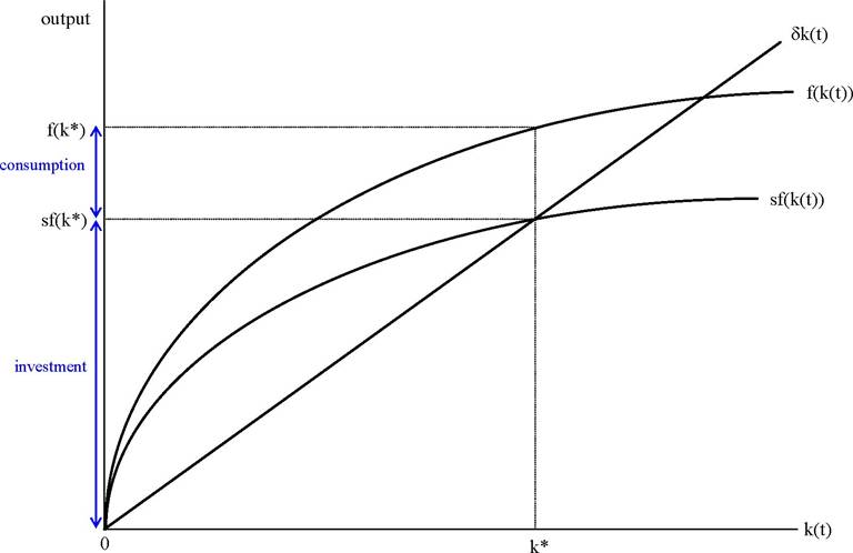
Figure 2.4. Investment and consumption in the steady-state equilibrium.
This analysis therefore leads to the following proposition (with the convention that the intersection at k = 0 is being ignored even when f (0) = 0):
PROPOSITION 2.2. Consider the basic Solow growth model and suppose that Assumptions 1 and 2 hold. Then, there exists a unique steady state equilibrium where the capital-labor ratio k* ∈ (0, ∞) is given by (2.18), per capita output is given by
and per capita consumption is given by
where the last equality uses (2.15). Since f (k) /k is everywhere (strictly) decreasing, there can only exist a unique value k* that satisfies (2.18).
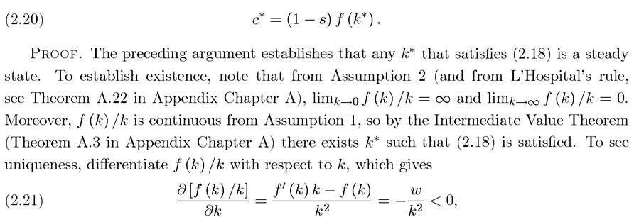
Figure 2.5. Examples of nonexistence and nonuniqueness of interior steady states when Assumptions 1 and 2 are not satisfied.
Equations (2.19) and (2.20) then follow by definition.
?
Figure 2.5 shows through a series of examples why Assumptions 1 and 2 cannot be dispensed with for the existence and uniqueness results in Proposition 2.2. In the first two panels, the failure of Assumption 2 leads to a situation in which there is no steady state equilibrium with positive activity, while in the third panel, the failure of Assumption 1 leads to non-uniqueness of steady states.
So far the model is very parsimonious: it does not have many parameters and abstracts from many features of the real world in order to focus on the question of interest. An understanding of how cross-country differences in certain parameters translate into differences in growth rates or output levels is essential for our focus. This will be done in the next proposition. But before doing so, let us generalize the production function in one simple way, and assume that
where A > 0, so that A is a shift parameter, with greater values corresponding to greater productivity of factors. Thistypeofproductivityisreferredtoas “Hicks-neutral” (see below). For now, it is simply a convenient way of looking at the impact of productivity differences across countries. Since f (k) satisfies the regularity conditions imposed above, so does f (k).
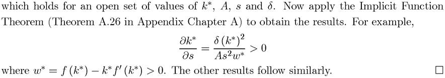
Therefore, countries with higher saving rates and better technologies will have higher capital-labor ratios and will be richer. Those with greater (technological) depreciation, will tend to have lower capital-labor ratios and will be poorer. All of the results in Proposition 2.3 are intuitive and they provide us with a first glimpse of the potential determinants of the capital-labor ratios and output levels across countries.
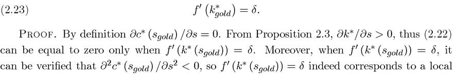
The same comparative statics with respect to A and δ immediately apply to c* as well. However, it is straightforward to see that c* will not be monotone in the saving rate (think, for example, of the extreme case where s = 1). In fact, there will exist a specific level of the saving rate, sgold, referred to as the “golden rule” saving rate, which maximizes the steadystate level of consumption. Since we are treating the saving rate as an exogenous parameter and have not specified the ob jective function of households yet, we cannot say whether the golden rule saving rate is “better” than some other saving rate. It is nevertheless interesting to characterize what this golden rule saving rate corresponds to.
To do this, let us first write the steady state relationship between c* and s and suppress the other parameters: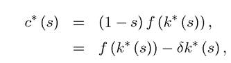
where the second equality exploits the fact that in steady state sf (k) = δk. Now differentiating this second line with respect to s (again using the Implicit Function Theorem), we have

Let us define the golden rule saving rate sgold to be such that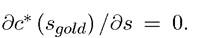 The
The
corresponding steady-state golden rule capital stock is defined as These quantities and the relationship between consumption and the saving rate are plotted in Figure 2.6.
The next proposition shows that sgol d and- are uniquely defined and the latter satisfies
(2.23).
PROPOSITION 2.4. In the basic Solow growth model, the highest level of steady-state consumption is reached for sgold. with the corresponding steady-state capital level k*old such that
48
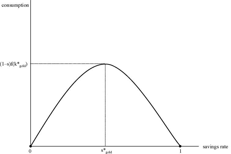
Figure 2.6. The “golden rule” level of savings rate, which maximizes steadystate consumption.
In other words, there exists a unique saving rate, sr,o∣r∣, and also a unique corresponding capital-labor ratio, maximizing the level of steady-state consumption. When the economy is below
 the higher saving rate will increase consumption, whereas when the economy is above
 steady-state consumption can be increased by saving less. In the latter case, lower savings translate into higher consumption because the capital-labor ratio of the economy is too high; individuals are investing too much and not consuming enough. This is the essence of what is referred to as dynamic inefficiency, which will be discussed in greater detail in Chapter 9. For now, recall that there is no explicit utility function here, so statements about “inefficiency” must the considered with caution. In fact, the reason why this type of dynamic inefficiency will not arise when consumption-saving decisions are endogenized may already be apparent to many of you.
2.3.