Transitional Dynamics in the Discrete Time Solow Model
Proposition 2.2 establishes the existence of a unique steady-state equilibrium (with positive activity). Recall that an equilibrium path does not refer simply to the steady state, but to the entire path of capital stock, output, consumption and factor prices.
This is an important point to bear in mind, especially since the term “equilibrium” is used differently in economics than in physical sciences. Typically, in engineering and physical sciences, an equilibrium refers to a point of rest of a dynamical system, thus to what I have so far referred to as the steady-state equilibrium. One may then be tempted to say that the system is in “disequilibrium” when it is away from the steady state. However, in economics, the non-steady-state behavior of an economy is also governed by market clearing and optimizing behavior of households and firms. Most economies spend much of their time in non-steadystate situations. Thus we are typically interested in the entire dynamic equilibrium path of the economy, not just its steady state.
I will refer to x* as a steady state of the difference equation (2.24).5 The relevant notion of stability is introduced in the next definition.
5Various other terms are used to describe xt, for example, “equilibrium point” or “critical point”. Since these other terms have different meanings in economics, I will refer to xt as a steady state throughout.
The next theorem provides the main results on the stability properties of systems of linear difference equations. The following theorems are special cases of the results presented in Appendix Chapter B.
Theorem 2.2. (Stability for Systems of Linear Difference Equations) Consider the following linear difference equation system

Unfortunately, much less can be said about nonlinear systems, but the following is a standard local stability result.
Theorem 2.3. (Local Stability for Systems of Nonlinear Difference Equations) Consider the following nonlinear autonomous system

An immediate corollary of Theorem 2.3 is the following useful result: 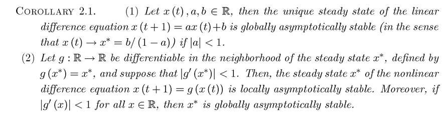
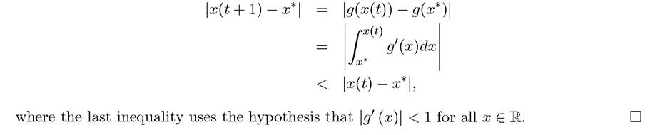
Proof. The first part follows immediately from Theorem 2.2. The local stability of g in the second part follows from Theorem 2.3. Global stability follows since
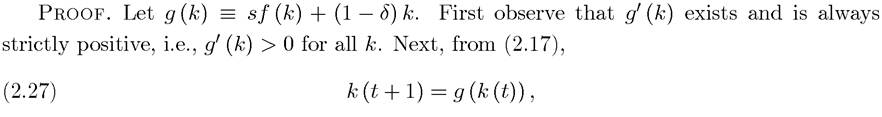
We can now apply Corollary 2.1 to the equilibrium difference equation of the Solow model,
(2.17):
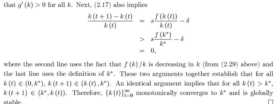
PROPOSITION 2.5. Suppose that Assumptions 1 and 2 hold, then the steady-state equilibrium of the Solow growth model described by the difference equation (2.17) is globally asymptotically stable, and starting from any k (0) > 0, k (t) monotonically converges to k*.
with a unique steady state at k*. From (2.18), the steady-state capital k* satisfies δk* = sf (k*), or

Now recall that f (∙) is concave and differentiable from Assumption 1 and satisfies f (0) ≥ 0 from Assumption 2. For any strictly concave differentiable function, we have

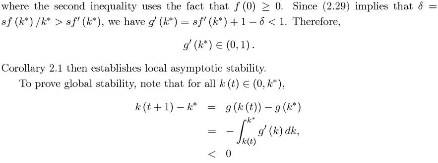
where the first line follows by subtracting (2.28) from (2.27), the second line uses the Fundamental Theorem of Calculus (Theorem B.2), and the third line follows from the observation 52
This stability result can be seen diagrammatically in Figure 2.7.
Starting from initial capital stock k (0) > 0, which is below the steady-state level k*, the economy grows towards k* and experiences capital deepening—meaning that the capital-labor ratio increases. Together with capital deepening comes growth of per capita income. If, instead, the economy were to start with it would reach the steady state by decumulating capital and contracting
 (that is, by experiencing negative growth).
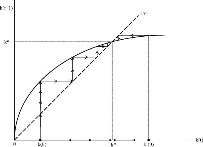
Figure 2.7. Transitional dynamics in the basic Solow model.
The following proposition is an immediate corollary of Proposition 2.5:
53
Proposition 2.6. Suppose that Assumptions 1 and 2 hold, and k (0) < k*, then  is an increasing sequence and
 is a decreasing sequence.
the opposite results apply.
Proof. See Exercise 2.9. ?
Recall that when the economy starts with too little capital relative to its labor supply, the capital-labor ratio will increase. This implies that the marginal product of capital will fall due to diminishing returns to capital and the wage rate will increase. Conversely, if it starts with too much capital, it will decumulate capital, and in the process the wage rate will decline and the rate of return to capital will increase.
The analysis has established that the Solow growth model has a number of nice properties; unique steady state, asymptotic stability, and finally, simple and intuitive comparative statics. Yet, so far, it has no growth. The steady state is the point at which there is no growth in the capital-labor ratio, no more capital deepening and no growth in output per capita. Consequently, the basic Solow model (without technological progress) can only generate economic growth along the transition path when the economy starts with k (0) < k*. However, this growth is not sustained: it slows down over time and eventually comes to an end. Section 2.7 will show that the Solow model can incorporate economic growth by allowing exogenous technological change. Before doing this, it is useful to look at the relationship between the discrete-time and continuous-time formulations.
2.4.