The Solow Model in Continuous Time
2.4.1. From Difference to Differential Equations. Recall that the time periods could refer to days, weeks, months or years. In some sense, the time unit is not important. This suggests that perhaps it may be more convenient to look at dynamics by making the time unit as small as possible, that is, by going to continuous time.
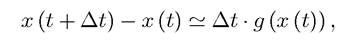
While much of modern macroeconomics (outside of growth theory) uses discrete-time models, many growth models are formulated in continuous time. The continuous-time setup has a number of advantages, since some pathological results of discrete-time models disappear in continuous time (see Exercise 2.16). Moreover, continuous-time models have more flexibility in the analysis of dynamics and allow explicit-form solutions in a wider set of circumstances. These considerations motivate a detailed study of both the discrete-time and the continuous-time versions of the basic models.Let us start with a simple difference equation

This equation states that between time t and t + 1, the absolute growth in x is given by g (x (t)). Let us now consider the following approximation
54
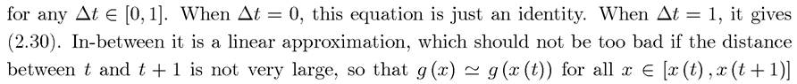
(however, you should also convince yourself that this approximation could in fact be quite bad if you take a very nonlinear function g, for which the behavior changes significantly between x (t) and x (t + 1)). Now divide both sides of this equation by ∆t, and take limits to obtain

where throughout the book I use the “dot” notation
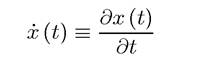
to denote time derivatives.
Equation (2.31) is a differential equation representing the same dynamics as the difference equation (2.30) for the case in which the distance between t and t + 1 is “small”.2.4.2. The Fundamental Equation of the Solow Model in Continuous Time. We can now repeat all of the analysis so far using the continuous-time representation. Nothing has changed on the production side, so we continue to have (2.6) and (2.7) as the factor prices, but now these refer to instantaneous rental rates. For example, w (t) is the flow of wages that workers receive at time t. Savings are again given by
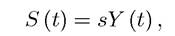
while consumption is still given by (2.11) above.
Let us also introduce population growth into this model, and assume that the labor force L (t) grows proportionally, that is,
(2.32)
The purpose of doing so is that in many of the classical analyses of economic growth, population growth plays an important role, so it is useful to see how it affects things here. There is still no technological progress.
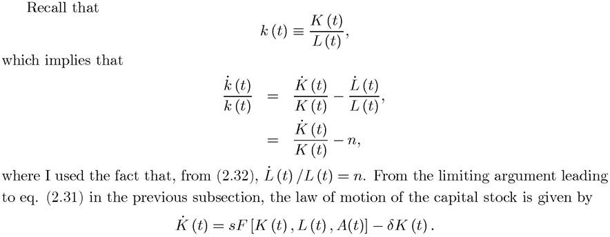
Using the definition of k (t) as the capital-labor ratio and the constant returns to scale properties of the production function, the fundamental law of motion of the Solow model in continuous time is obtained as

where, following usual practice, I have transformed the left-hand side to the proportional change in the capital-labor ratio by dividing both sides by k (t).6
As before, a steady-state equilibrium involves k (t) remaining constant at some level k*. It is easy to verify that the equilibrium differential equation (2.33) has a unique steady state at k*, which is given by a slight modification of (2.18) above to incorporate population growth:

In other words, going from discrete to continuous time has not changed any of the basic economic features of the model, and again the steady state can be plotted in a diagram similar to the one used above (now with the population growth rate featuring in there as well).
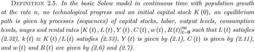
This is done in Figure 2.8, which also highlights that the logic of the steady state is the same with population growth as it was without population growth. The amount of investment, sf (k), is used to replenish the capital-labor ratio, but now there are two reasons for replenishments. The capital stock depreciates, again exponentially, at the flow rate δ. In addition, the capital stock must also increase as population grows in order to maintain the capital-labor ratio at a constant level. The amount of capital that needs to be replenished is therefore (n + δ) k.PROPOSITION 2.7. Consider the basic Solow growth model in continuous time and suppose that Assumptions 1 and 2 hold. Then, there exists a unique steady state equilibrium where the capital-labor ratio is equal to k* ∈ (0, ∞) and is given by (2.34), per capita output is given by 
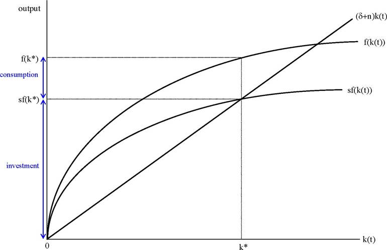
Figure 2.8. Investment and consumption in the state-state equilibrium with population growth.
and per capita consumption is given by
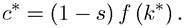
PROOf. See Exercise 2.5.

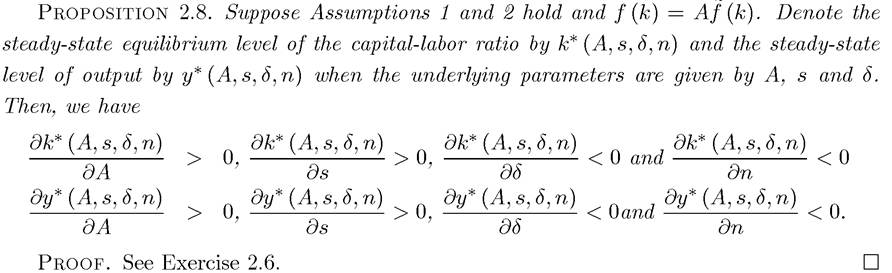
The new result relative to the earlier comparative static proposition is that now a higher population growth rate, n, also reduces the capital-labor ratio and output per capita. The reason for this is simple: a higher population growth rate means there is more labor to use the existing amount of capital, which only accumulates slowly, and consequently the equilibrium capital-labor ratio ends up lower. This result implies that countries with higher population growth rates will have lower incomes per person (or per worker).
2.5.