Transitional Dynamics in the Continuous Time Solow Model

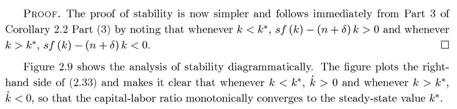
The analysis of transitional dynamics and stability with continuous time yields similar results to those in Section 2.3, but the analysis will be slightly simpler. Let us first recall the basic results on the stability of systems of differential equations.

Theorem 2.4. (Stability of Linear Differential Equations) Considerthefollowing linear differential equation system

(2.35)

Once again an immediate corollary is:

58

Proof. See Exercise 2.10.

?

Notice that the equivalent of the Part 3 of Corollary 2.2 is not true in discrete time, and this will be illustrated in Exercise 2.16.

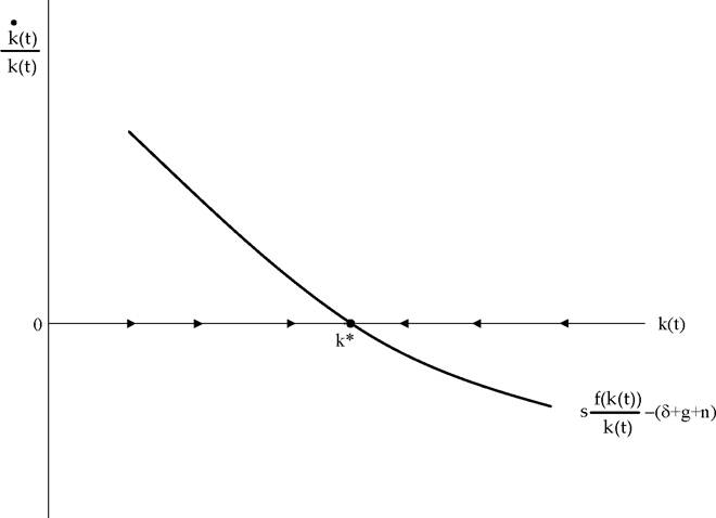
Figure 2.9. Dynamics of the capital-labor ratio in the basic Solow model.

In view of these results, Proposition 2.5 immediately generalizes:

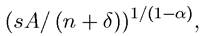
PROPOSITION 2.9. Suppose that Assumptions 1 and 2 hold, then the basic Solow growth model in continuous time with constant population growth and no technological change is globally asymptotically stable, and starting from any k (0) > 0, k (t) monotonically converges to k*.

59

Similarly, the share of labor is (t) = 1 — α. The reason for this is that with an elasticity of substitution equal to 1, as capital increases, its marginal product decreases proportionally, leaving the capital share (the amount of capital times its marginal product) constant.

Recall that with the Cobb-Douglas technology, the per capita production function takes the form f (k) = Ak^α, so the steady state is given again from (2.34) (with population growth

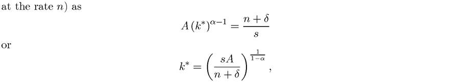
which is a simple expression for the steady-state capital-labor ratio. It immediately follows that k* is increasing in s and A, and decreasing in n and δ (and these results are naturally consistent with those in Proposition 2.8). In addition, k* is increasing in α. This is because a higher α implies less diminishing returns to capital, thus a higher capital-labor ratio is necessary to reduce the average return to capital to a level consistent with steady state as given in eq. (2.34).

Transitional dynamics are also straightforward in this case. In particular,

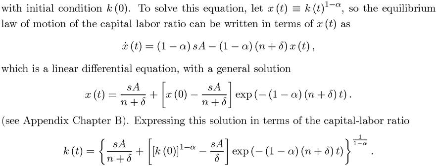
This solution illustrates that starting from any k (0), the equilibrium=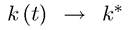

and in fact, the rate of adjustment is related to (1 — α)(n + δ). More specifically, the gap between k (0) and the steady-state value k* narrows at the exponential rate (1 — α)(n + δ). This is intuitive: a higher α implies less diminishing returns to capital, which slows down the rate at which the marginal and average product of capital decline as capital accumulates, and this reduces the rate of adjustment to steady state. Similarly, a smaller δ means less replacement of depreciated capital and a smaller n means slower pop­ulation growth, and both of those slow down the adjustment of capital per worker and thus the rate of transitional dynamics.

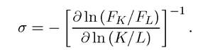
EXAMPLE 2.3. (The Constant Elasticity of Substitution Production Function) The previous example introduced the Cobb-Douglas production function, which featured an elasticity of substitution equal to 1. The Cobb-Douglas production function is a special case of the constant elasticity of substitution (CES) production function, first introduced by Arrow, Chenery, Minhas and Solow (1961). This production function imposes a con­stant elasticity, σ, not necessarily equal to 1. Consider a vector-valued index of technology 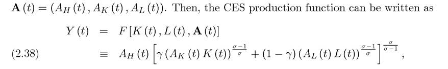where Ah (t) > 0, Ak (t) > 0 and Al (t) > 0 are three different types of technological change which will be discussed further in Section 2.7; γ ∈ (0,1) is a distribution parameter, which determines how important labor and capital services are in determining the production of the final good and σ ∈ [0, ∞] is the elasticity of substitution. To verify that σ is indeed the constant elasticity of substitution, let us use (2.37). In particular, it is easy to verify that the ratio of the marginal product of capital to the marginal productive labor, Fk/Fl, is given by

so that the elasticity of substitution is indeed given by σ, that is,

The CES production function is particularly useful because it is more general and 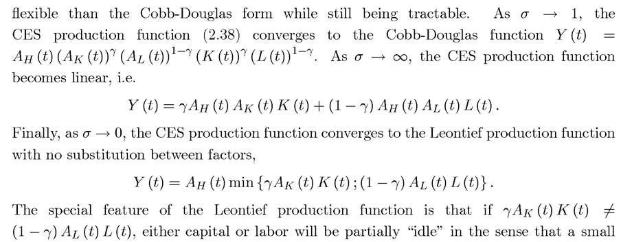reduction in capital or labor will have no effect on output or factor prices. Exercise 2.18 illustrates a number of the properties of the CES production function, while Exercise 2.19 provides an alternative derivation of this production function along the lines of the original article by Arrow, Chenery, Minhas and Solow (1961). Finally, an important observation is that the CES production function with σ > 1 violates Assumption 1 (see Exercise 2.20).

Therefore, in the context of aggregate production functions with capital and labor, σ ≤ 1 is the natural assumption.

2.6.