Wage Determination and Equilibrium Unemployment
In equilibrium, this model determines the three endogenous variables u, θ, and w, which simultaneously satisfy the Beveridge curve (18.8), the job creation condition (18.17), and the wage equation (18.33).
The full model is thus given by
From the last two equations, we can establish that the level of real wages w and labor market tightness θ can be determined independently of the unemployment rate u. The job creation condition and the wage equation suffice for the determination of real wages and labor market tightness. Once we determine labor market tightness θ, we can substitute for it in the Beveridge curve (18.8) and determine equilibrium unemployment.
The determination of equilibrium real wages and labor market tightness is presented in figure 18.3. The wage equation (18.33) implies a positive relation between the real wage and labor market tightness. The job creation condition (18.17) implies a negative relation between the real wage and labor market tightness. Equilibrium real wages and labor market tightness are determined at the intersection of these two curves.
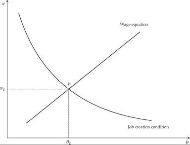
Figure 18.3 The determination of real wages and labor market tightness.
As shown in the figure, the wage function has a positive slope, because the higher labor market tightness is, the higher will be the wage that prospective employees can negotiate with employers. The job creation condition has a negative slope, because higher wages make creating vacancies less profitable and thus reduce vacancies relative to unemployment. We also see that the determination of real wages and labor market tightness do not depend on the unemployment rate. This is because of the assumption of constant returns to scale in the matching function.
Once θ is determined from the wage equation and the job creation condition, we can substitute it in the Beveridge curve (18.8) and determine the unemployment rate. The solution is shown in figure 18.1.
In figure 18.1, the positively sloped straight line has a slope of θE, the equilibrium ratio of vacancies to the unemployed, as analyzed in figure 18.3. The negatively sloped Beveridge curve is derived from equation (18.8), which equates the flows in and out of unemployment. Higher vacancies imply lower unemployment, because the probability of finding a job by an unemployed job seeker is higher. The curve is convex to the origin because of the properties of the matching function. The equilibrium unemployment rate is determined at the intersection of the Beveridge curve with the straight line through the origin, the slope of which is determined by labor market tightness.
18.7