Determinants of Equilibrium Unemployment, Real Wages, and Labor Market Tightness

We can now use the full model to examine how real wages, labor market tightness, and equilibrium unemployment depend on the various exogenous parameters and shocks.

18.7.1 An Increase in Labor Productivity

Let us first consider a permanent increase in labor productivity p.

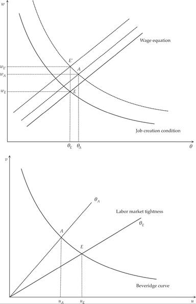
Figure 18.4 Labor productivity and equilibrium unemployment.

This effect of labor productivity occurs because of the assumption that the unemployment benefit z is fixed and does not depend on labor productivity. In this case, changes in real wages do not fully reflect changes in labor productivity. Thus, when productivity increases, there are gains from the creation of new job vacancies, new vacancies are then created, and unemployment falls.

However, in many countries, unemployment benefits z are not fixed in real terms and usually are related to the real wages of the employed. Thus, the assumption of an exogenously fixed unemployment benefit z is not very realistic.

Moreover, if the prediction that the growth of labor productivity reduces the unemployment rate is correct, then unemployment would be tending toward zero in the long run because of the continuous increases in labor productivity resulting from economic growth. This prediction is not compatible with the existing empirical evidence, which does not suggest any long-run trends in unemployment rates.

Assuming that unemployment benefits z are a percentage ρ of real wages, where 0 < ρ < 1, then in our model, we have that z = ρw; ρ is usually called the replacement rate.

In this case, the wage function (18.33) is converted to

With the assumption of an exogenous replacement rate, the wage equation (18.33) becomes proportional to labor productivity p. The factor of proportionality depends positively on the bargaining power of prospective employees β, labor market tightness θ, the cost of maintaining a vacancy c, and the replacement rate of the unemployment benefit system ρ.

For a given labor market tightness, an increase (or fall) in labor productivity results in an equiproportional shift in the wage equation.

From the job creation condition (18.17), a rise in productivity also results in an equiproportional shift in the real wage that satisfies the job creation condition for a given labor market tightness.

This case is also presented in figure 18.4. An increase in labor productivity moves the wage equation and the job creation condition by the same proportion, thus increasing real wages without affecting the degree of labor market tightness. Consequently, the unemployment rate is not affected by an increase in labor productivity in the case where the unemployment benefit is proportional to real wages.

Another way to see the independence of labor market tightness from labor productivity when the unemployment benefit is proportional to the real wage is to equate the right-hand sides of (18.17) and (18.33):

Equation (18.35) implies that in equilibrium, labor market tightness is independent of labor productivity.

The independence of labor market tightness (and therefore the equilibrium unemployment rate) from average labor productivity is a desirable property, because unemployment rates do not display a long-term trend, as would be the case if they depended on increases in labor productivity, which have an upward long-term trend.

18.7.2 An Increase in Unemployment Benefits

We can also examine the implications of an increase in unemployment benefits z (or in the case z = ρw, an increase in the replacement rate ρ). This causes an increase in real wages, reduces labor market tightness, and results in higher equilibrium unemployment.

The relevant analysis is shown in figure 18.5. An increase of z (or ρ in the case z = ρw) shifts the wage equation upward, because prospective workers demand higher wages, given that the cost of unemployment is now lower.

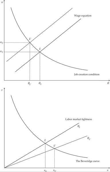
Figure 18.5 Unemployment benefits and equilibrium unemployment.

When wages are higher, firms create fewer jobs through the job creation condition. Consequently, the unemployment rate increases, and the vacancy rate decreases.

An increase of β, the relative bargaining power of job seekers, would have the same impact for similar reasons. Real wages rise, and labor market tightness is reduced. Consequently, the unemployment rate rises, and the vacancy rate decreases from the Beveridge curve.

18.7.3 An Increase in the Real Interest Rate

Figure 18.6 shows the impact of an exogenous increase in the real interest rate. An increase in the real interest rate shifts the job creation condition in figure 18.6 to the left, as it increases the cost of maintaining vacancies. This results in a reduction of both real wages and labor market tightness.

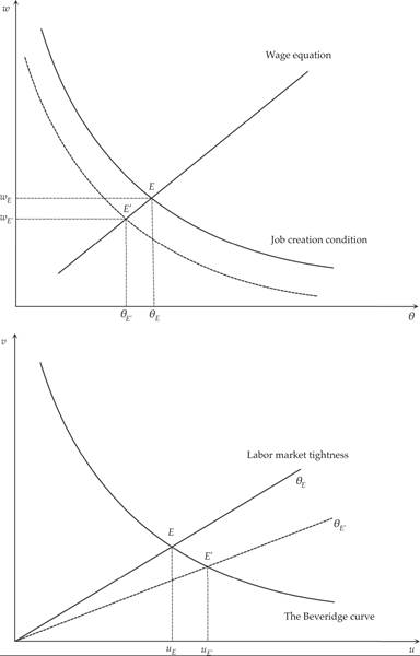
Figure 18.6 The real interest rate and equilibrium unemployment.

The reason is that with a higher real interest rate, expected future revenues from the creation of a new job have a lower present value, but the cost of creating the new job is paid up front. Therefore, there is less of an incentive to create new jobs. The fall in labor market tightness naturally leads to an increase in the unemployment rate through the Beveridge curve (figure 18.6b).

18.7.4 An Increase in the Probability of Job Destruction

Finally, let us analyze the implications of an increase in λ, the exogenous probability of termination of a job. This case is depicted in figure 18.7.

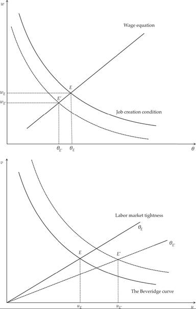
Figure 18.7 The probability of job destruction and equilibrium unemployment.

An increase in λ leads to a reduction in real wages and labor market tightness, because it reduces the expected revenue from the creation of a new job. Consequently, fewer job vacancies are created, labor market tightness is reduced, and flows from unemployment to jobs decrease. This leads to an increase in the unemployment rate (figure 18.7, top).

In this case, equilibrium unemployment also increases, because flows into unemployment also rise. An increase in λ shifts the Beveridge curve to the right (figure 18.7, bottom), as flows from existing jobs to unemployment rise. Consequently, equilibrium unemployment increases both because of the increase of flows from employment to unemployment (resulting directly from the rise of λ) and because of the decrease of flows from unemployment to jobs (resulting from the fall in labor market tightness θ). The impact of an increase in λ on the equilibrium vacancy rate is uncertain, because it depends on the exact values of the parameters of the model.

Thus, the theoretical analysis implies an increase in equilibrium unemployment following a rise in unemployment benefits (or the replacement ratio), real interest rates, and the probability of job destruction. The reason is that all these shocks reduce labor market tightness and the vacancy rate, reducing flows from unemployment to jobs. In addition, an increase in the probability of job destruction also increases flows from jobs to unemployment, further increasing equilibrium unemployment.