18.8 Dynamic Adjustment to the Steady State

Our analysis so far has concentrated on the determination of equilibirum, or steady state, unemployment; almost nothing has been said about the dynamic adjustment of the labor market in the short run.

Assume that vacancies and real wages are non-predetermined variables, because they depend on forward-looking expectations of firms and job seekers. Also assume that unemployment is a predetermined variable, governed by equation (18.6). Then we can show that there is a unique saddle path that leads unemployment to its equilibrium or steady state value.

18.8.1 The Dynamic Adjustment of Unemployment and Vacancies

From (18.6), the unemployment rate evolves according to

where θ_E is the equilibrium labor market tightness determined through the wage negotiations of firms with vacancies and unemployed job seekers, which was analyzed in the previous sections. Because vacancies are a non-predetermined variable, and θ is determined independently of the unemployment rate, θ and real wages w jump immediately to their equilibrium values.

From the solution of the differential equation (18.36), the short-run evolution of unemployment is determined by

where u₀ is the unemployment rate at time 0, and u_E is the steady state unemployment rate, defined as

From (18.37), the unemployment rate will converge to its steady state value from any initial rate, with a speed of adjustment equal to λ + θ_Eq(θ_E).

Because θ_E remains constant along the adjustment path, vacancies will be adjusting at the same rate as unemployment along the adjustment path, implying that

The relevant phase diagram in vacancy-unemployment space is shown in figure 18.8. We assume that the labor market is originally in steady state equilibrium (v₀, u₀), and there is a unanticipated permanent shock that changes θ to θ_E. We assume that θ_E implies a higher steady state unemployment rate u_E and a lower steady state vacancy rate v_E. How will the labor market adjust?

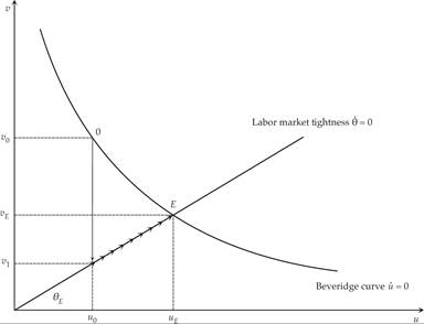
Figure 18.8 Dynamic adjustment of unemployment and vacancies.

As can be seen from the phase diagram in figure 18.8, vacancies, which are the non-predetermined variable, will jump from v₀ to v₁. There will be an immediate drop in vacancies to ensure that labor market tightness jumps to its new steady state value. Following that, both the unemployment rate and the vacancy rate will gradually adjust upward toward their new steady state values, as described by the differential equations (18.33) and (18.36). Because the unemployment rate is a predetermined variable, the non-predetermined vacancy rate initially overshoots its steady state drop.

Thus, this model explains not only the steady state unemployment rate (i.e., the natural rate of unemployment) but also the dynamic adjustment process of the unemployment rate toward its natural rate, following shocks to the determinants of equilibrium wages and equilibrium tightness in the labor market.

The model has been extended, and applied and tested extensively. An early test the model for unemployment in Britain is in Pissarides [1986]. Blanchard and Diamond [1989, 1990] and Shimer [2005], among others, have estimated and tested the model for US data, with generally mixed results. Merz [1995] and Andolfatto [1996] have introduced the model into an RBC framework with intertemporal substitution of leisure and capital accumulation.

18.8.2 Numerical Simulations of the Model

To get a quantitative sense of the extent to which shifts in the various parameters affect the equilibrium unemployment rate, real wages, and labor market tightness, it is worth simulating the model numerically. The simulations presented here assume that the matching function is Cobb-Douglas with constant returns to scale and is described by

where M > 0 is the efficiency of the matching process, and 0 < μ < 1 is the elasticity of job creation with respect to unemployment.

From (18.40), the probability of filling a vacancy is determined by

Substituting (18.41) in the Beveridge curve (18.8) and the job creation condition (18.17), the model takes the form

The simulation assumes the following initial parameter values: λ = 2.5%, M = 1/2, μ = 1/2, p = 1, c = 1/2, r = 3%, ρ = 1/2, and β = 1/2. Simulating the model for these parameter values, we get w = 0.95, θ = 0.85, u = 5.1%, and v = 4.4%.

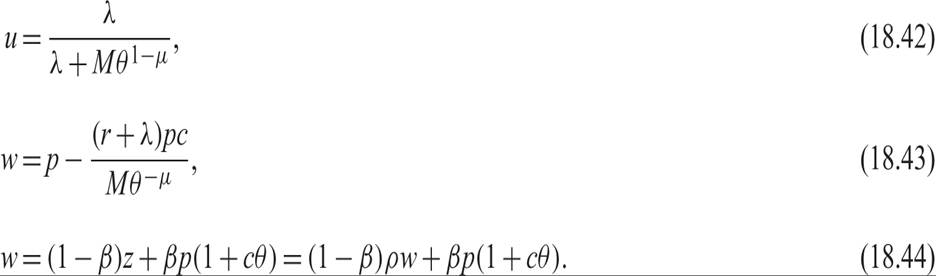
The real wage is 95% of productivity and the unemployment rate is relatively low at 5.1%. If the probability of job destruction λ were to double to 5%, then it follows that w = 0.93, θ = 0.79, u = 10.1%, and v = 7.9%.

Relative to the original equilibrium, the real wage falls by 2.1%, to 93% of productivity, and the natural rate of unemployment almost doubles, to 10.1%.

The dynamic adjustment of the unemployment rate and the vacancy rate is depicted in figure 18.9. The vacancy rate initially falls and then starts rising as the unemployment and vacancy rates gradually rise toward their higher equilibrium values.

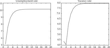
Figure 18.9 Dynamic adjustment of unemployment and vacancies to an increase in the job destruction rate.

If the replacement ratio ρ were to rise from 0.5 to 0.7 (a 40% increase), then it follows that w = 0.96, θ = 0.50, u = 6.6%, and v = 3.3%.

Relative to the original equilibrium, the real wage rises by roughly 1%, and the unemployment rate rises by 1.5 percentage points, to 6.6%. With a constant labor force, this is equivalent to a 29.4% rise in the number of the unemployed.

The dynamic adjustment of the unemployment rate and the vacancy rate is depicted in figure 18.10. Note the overshooting of the fall in the vacancy rate, relative to its steady state fall, which conforms with the theoretical analysis in figure 18.8. Because of the fall in equilibrium labor market tightness, the vacancy rate initially falls. As the unemployment rate gradually rises toward its higher new steady state value, the vacancy rate gradually rises as well. Thus, the short-run reduction in the vacancy rate exceeds the steady state reduction.

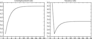
Figure 18.10 Dynamic adjustment of unemployment and vacancies to an increase in the replacement rate.

Finally, if the real interest rate r were to double from the original 3% to 6%, it follows that w = 0.925, θ = 0.78, u = 5.4%, and v = 4.2%.

Relative to the initial equilibrium, the real wage falls by about 2.5%, and the unemployment rate rises by 0.3 percentage points, to 5.4%.

The dynamic adjustment of the unemployment rate and the vacancy rate is depicted in figure 18.11. Note again the overshooting of the fall of the vacancy rate.

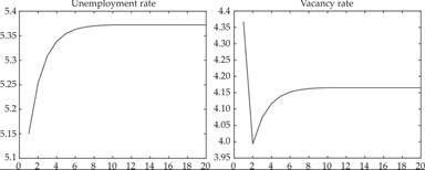
Figure 18.11 Dynamic adjustment of unemployment and vacancies to an increase in the real interest rate.

We see from these simulations (for the specific values of the parameters chosen) that shifts in the probability of job destruction—as well as shifts of the replacement rate of unemployment benefits—have relatively large effects on the equilibrium unemployment rate and relatively small effects on real wages. However, changes in the real interest rate have a relatively modest effect on both real wages and the unemployment rate.

18.9