Welfare Theorems
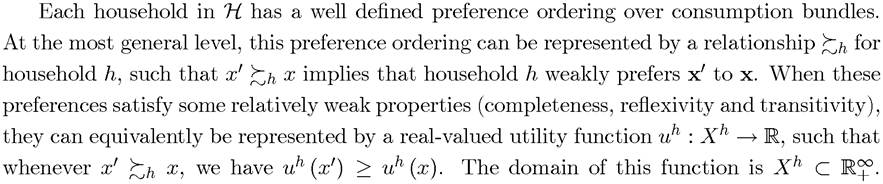
We are ultimately interested in equilibrium growth. But there is a close connection between Pareto optima and competitive equilibria. These connections could not be exploited in the preceding chapters, because household (individual) preferences were not specified.
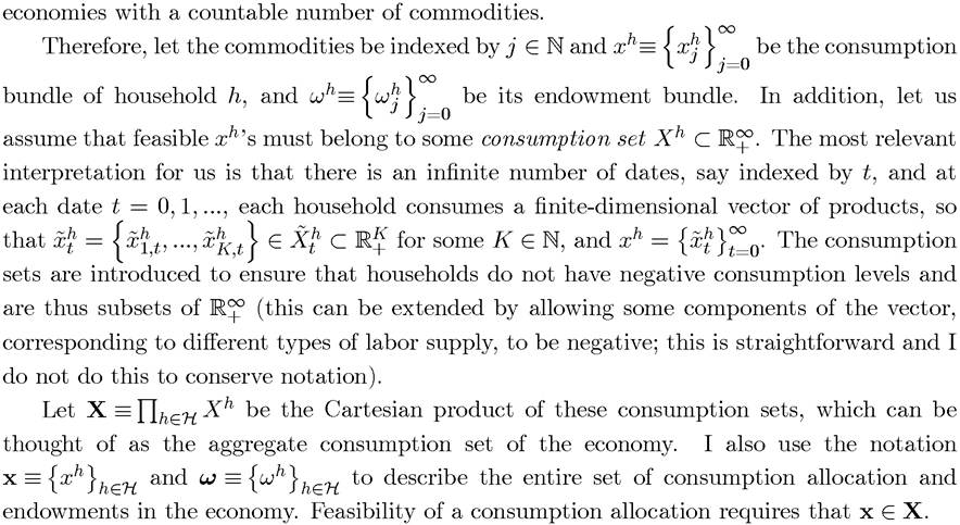
I now introduce the First and Second Welfare Theorems and develop the relevant connections between the theory of economic growth and dynamic general equilibrium models.Let us start with models that have a finite number of consumers, so that in terms of the notation above, the set H is finite. Throughout, I allow an infinite number of commodities, since dynamic growth models almost always feature an infinite number of time periods,
thus an infinite number of commodities. The results stated in this section have analogs for economies with a continuum of commodities (corresponding to dynamic economies in continuous time), but for the sake of brevity and to reduce technical details, I focus on
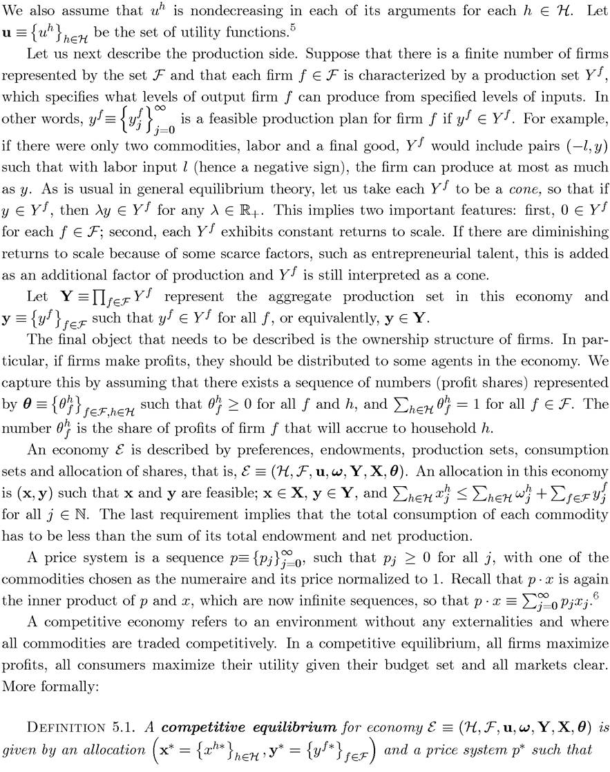
5Notice that despite the same notation, u, utility functions here are not instantaneous utility functions or felicity functions as in Section 5.1, but they are defined over the entire sequence of consumption bundles.
6You may note that such an inner product may not always exist in infinite dimensional spaces. This technical detail is dealt with in the proof of Theorem 5.7 below.
A major focus of general equilibrium theory is to establish the existence of a competitive equilibrium under reasonable assumptions.
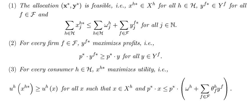
When there is a finite number of commodities and standard convexity assumptions are made on preferences and production sets, this is straightforward (in particular, the proof of existence involves simple applications of Theorems A.16, A.17, and A.19 in Appendix Chapter A). When there is an infinite number of commodities, as in infinite-horizon growth models, proving the existence of a competitive equilibrium is somewhat more difficult and requires more sophisticated arguments. Nevertheless, for our focus here proving the existence of a competitive equilibrium under general conditions is not central (since the typical growth models will have sufficient structure to ensure the existence of a competitive equilibrium in a relatively straightforward manner). Instead, the efficiency properties of competitive equilibria, when they exist, and the decentralization of certain desirable (efficient) allocations as competitive equilibria are more important. For this reason, let us recall the standard definition of Pareto optimality.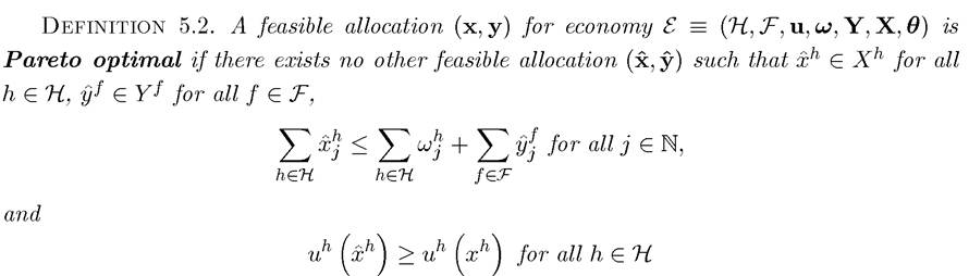
with at least one strict inequality in the preceding relationship.
184
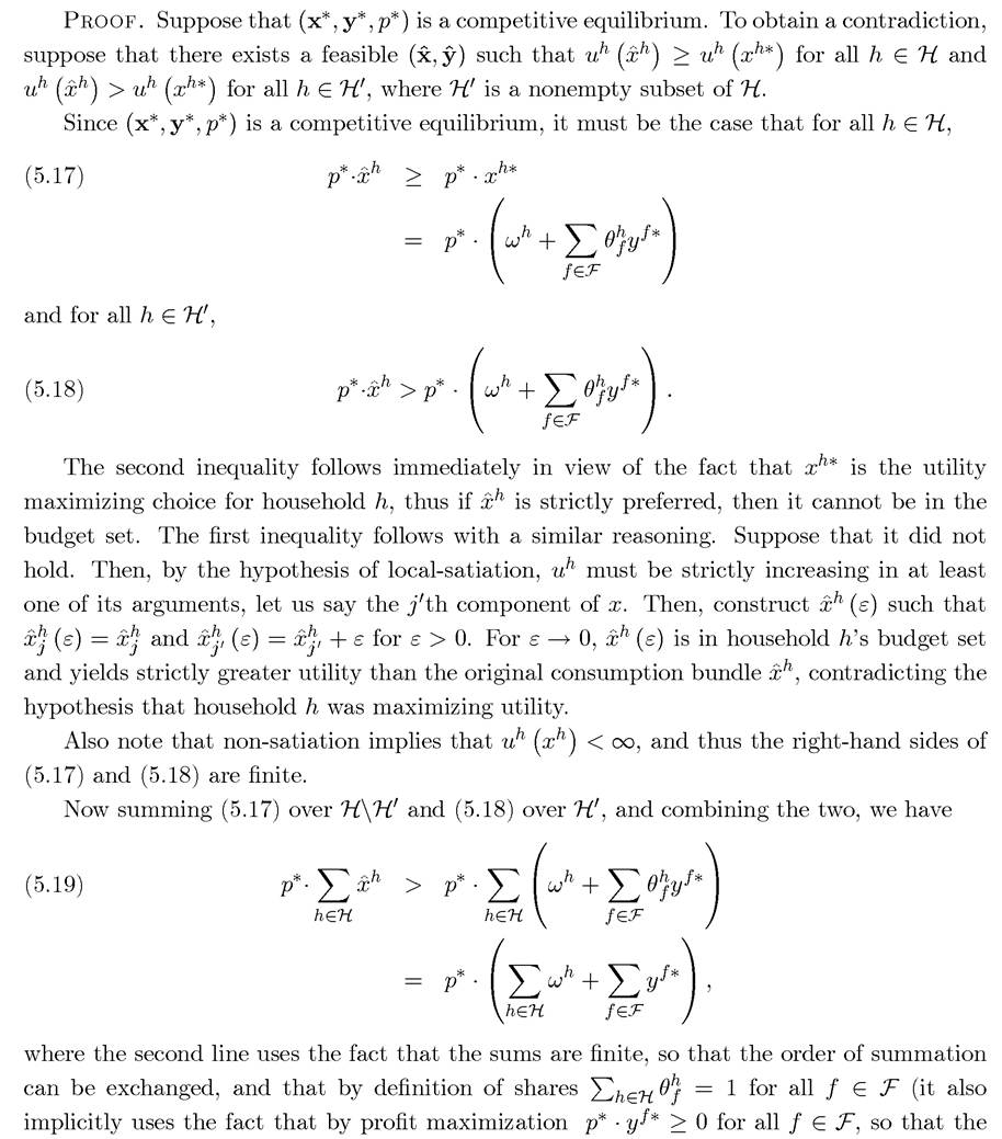
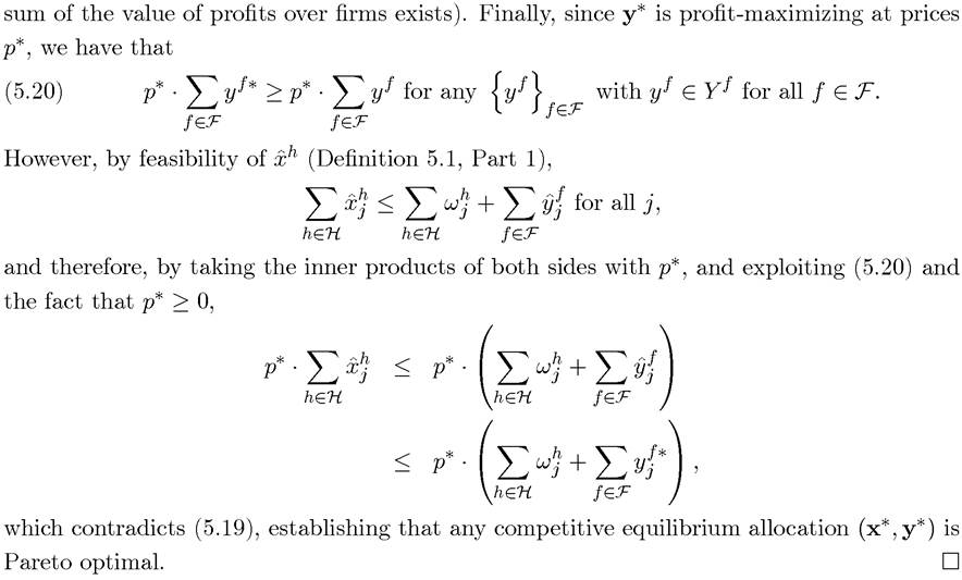
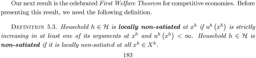
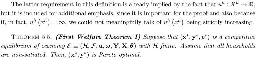
The proof of the First Welfare Theorem is both intuitive and simple. The proof is based on two intuitive ideas. First, if another allocation Pareto dominates the competitive equilibrium, then it must be non-affordable in the competitive equilibrium for at least one household. Second, profit-maximization implies that any competitive equilibrium already maximizes the set of affordable allocations.
It is also simple since it only uses the summation of the values of commodities at a given price vector. In particular, it makes no convexity assumption. However, the proof also highlights the importance of the feature that the relevant sums exist and are finite. Otherwise, the last step would lead to the conclusion that tζ∞ < ∞,5 which may or may not be a contradiction. The fact that these sums exist, in turn, followed from two assumptions: finiteness of the number of individuals and non-satiation. However, as noted before, working with economies that have only a finite number of households (even if there is an infinite number of commodities) is not always sufficient for our purposes. For this reason, the next theorem turns to the version of the First Welfare Theorem with an infinite number of households. For simplicity, here I take H to be a countably infinite set, e.g., H = N. The next theorem generalizes the First Welfare Theorem to this case. It makes use of an additional assumption to take care of infinite sums.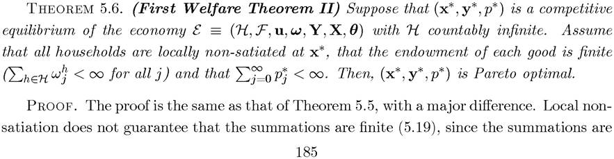

Theorem 5.6 will be particularly useful in the analysis of overlapping generation models in Chapter 9.
Let us next briefly discuss the Second Welfare Theorem, which is the converse of the First Welfare Theorem. It answers the question of whether a Pareto optimal allocation can be decentralized as a competitive equilibrium. Interestingly, for the Second Welfare Theorem whether or not H is finite is not as important as for the First Welfare Theorem. Nevertheless, the Second Welfare Theorem requires a number of assumptions on preferences and technology, such as the convexity of consumption and production sets and of preferences, and a number of additional technical requirements (which are trivially satisfied when the number of commodities is finite).
This is because the Second Welfare Theorem implicitly contains an “existence of equilibrium argument,” which runs into problems in the presence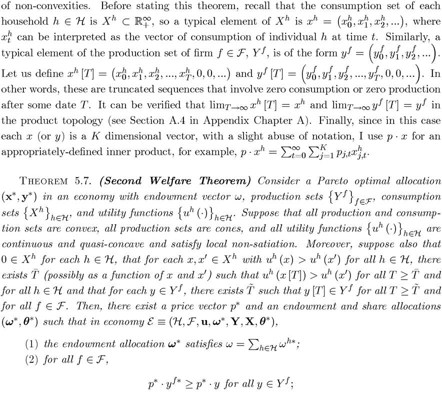
c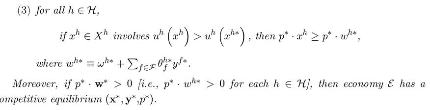
The proof of this theorem involves the application of the Geometric Hahn-Banach Theorem, Theorem A.28, from Appendix Chapter A. It is somewhat long and involved. For this reason, a sketch of this proof is provided in the next (starred) section. Here notice that if instead of an infinite-dimensional economy, we were dealing with an economy with a finite  of the Second Welfare Theorem in economies with a finite number of commodities. Its role in dynamic economies is that changes in allocations that are very far in the future should not have a “large” effect on preferences. This is naturally satisfied when we look at infinitehorizon economies with discounted utility and separable production structure. Intuitively, if a sequence of consumption levels x is strictly preferred to x', then setting the elements of x and x' to 0 in the very far (and thus heavily discounted) future should not change this conclusion (since discounting implies that x could not be strictly preferred to x0 because of higher consumption under x in the arbitrarily far future). Similarly, if some production vector y is feasible, the separable production structure implies that y [T], which involves zero production after some date T, must also be feasible. Exercise 5.13 demonstrates these claims more formally. One difficulty in applying this theorem is that uh may not be defined when x has zero elements (so that the consumption set Xh does not contain 0). Exercise 5.14 shows that the theorem can be generalized to the case in which there exists a strictly positive vector ε ∈ Rk with each element sufficiently small and with (ε,..., ε) ∈ Xh for all h ∈ H.
The conditions for the Second Welfare Theorem are more difficult to satisfy than those for the First Welfare Theorem because of the convexity requirements. In many ways, it is also the more important of the two theorems. While the First Welfare Theorem is celebrated as a formalization of Adam Smith’s invisible hand, the Second Welfare Theorem establishes the stronger result that any Pareto optimal allocation can be decentralized as a competitive equilibrium. An immediate corollary of this is an existence result; since the Pareto optimal allocation can be decentralized as a competitive equilibrium, a competitive equilibrium must exist (at least for the endowments leading to Pareto optimal allocations).
The Second Welfare Theorem motivates many macroeconomists to look for the set of Pareto optimal allocations instead of explicitly characterizing competitive equilibria. This is 187
especially useful in dynamic models where sometimes competitive equilibria can be quite difficult to characterize or even to specify, while the characterization of Pareto optimal allocations is typically more straightforward.
The real power of the Second Welfare Theorem in dynamic macro models comes when we combine it with models that admit a representative household. Recall that Theorem 5.3 shows an equivalence between Pareto optimal allocations and optimal allocations for the representative household. In certain models, including many—but not all—growth models studied in this book, the combination of a representative household and the Second Welfare Theorem enables us to characterize the optimal growth allocation that maximizes the utility of the representative household and assert that this will correspond to a competitive equilibrium.
5.7.