CONTRACT MECHANISMS PRODUCING FINANCIAL EVENTS
Financial contracts range from maturity loans to indices and some derivatives. In light of what we have just learned about constructing financial deals, it is easy to imagine that an unlimited number of possible contracts exist.
In fact, if you ask even people in the financial sector about their estimate of the number of different financial contracts in existence, they will often answer something along the lines “hundreds,” or “thousands.” Surprisingly enough, there are only three dozen types of financial contract that are able to map more than 98% of today's financial instruments. A well known financial contract is the annuity, used in many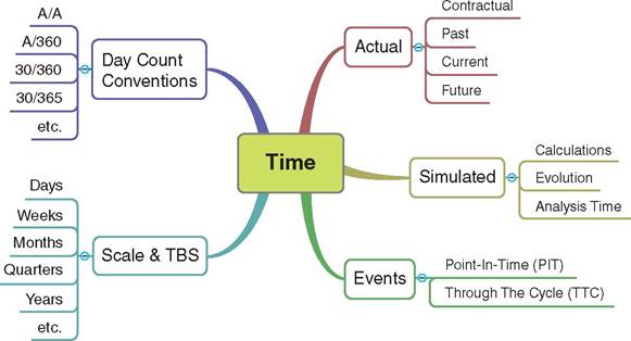
FIGURE 5.2 Main elements referring to time
loans in banking and P2P financial portfolios, principal at maturity (used in bonds), stocks, commodities, credit lines, etc. combination of them defining the derivative contracts. The mapping of such contracts is based on the elements discussed in Part Two of this book, and is illustrated in Figure 5.1. The reader can find a detailed description of the main contract types in other publications such as the textbook Unified Financial Analysis,3 also under the Algorithmic Contract Types Unified Standards project.4
All contracts follow several fundamental patterns based on the contract rules and algorithmic mechanism, all combining to generate the financial events. In other words, we are describing financial contracts mathematically by using functions considering fixed or variable:
■ Rule parameters, such as on payment and interest amounts, option of withdrawal of capital, etc.,
■ Points in time (PITs) and through-the-cycle (TTC) iterations, applied for instance on re-pricing, times of payments, etc.
Thus, we can from now on identify and analyze the events based on the combination of the above factors.
Note that patterns are in most cases interacting with, and interdepending on, each other; for instance, interest payments are based on principal amount and time of re-pricing. Table 5.1 illustrates the different combinations considered in the construction of the patterns for the financial events.TABLE 5.1 Contractual rules and parameters applied within fixed and variable times
| Time | |||||
| Fixed | Variable | ||||
| PIT | TTC | PIT | TTC | ||
| Rule parameters | Fixed Variable | Type I Type V | Type II Type VI | Type III Type VII | Type IV Type VIII |
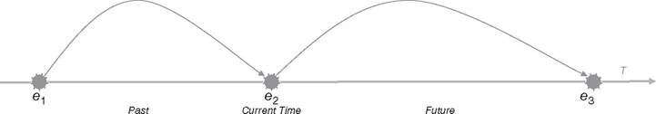
FIGURE 5.3 Past, current and future events according to time analysis
Types I and II define the events that are driven by rules with certain fixed parameters at times. Examples of such events are the defined (fixed) amount in principal payment of capital investment at the (fixed) PIT of value date (Type I), fixed interest rates and fixed principals (increase or decrease) paid TTC at fixed intervals (Type II).
A combination of fixed parameters arising through variable times fall into Types III and IV of event generation. Typical cases of such events are the predetermined fixed rates used in case of prepayment at any future PIT (Type III); another case could be a fixed interest rate applied through the cycles of payments that may be shifted to earlier or later time points (Type IV).
Cases where events result in variable parameters' of rules applied at fixed times fall into Types V and VI.
Variable interest rates and payments at maturity date PIT or at fixed TTC iterations are typical examples of these types.The most complex combinations are the ones where both rules and times that generate the events are variable (defined in Type VII and VIII). The degree of prepayment amount or use of a facility at any future PIT, based on a counterparty's decision, is a characteristic case of Type VII. Type VIII can be the case where variable interest rates and principal amounts (for instance, in an annuity contract) define the increase in payments and/or the maturity date, which may affect the corresponding increase and decrease in the cycle of payments.
In addition, we should identify whether the performances of the financial events are actual, expected, or unexpected. The first type, actual, is derived from the past historical events up to the current time, e.g., e1 and e2 shown in Figure 5.3. The expected and unexpected are referring to future events, e.g., e3 shown in Figure 5.3, and are estimated based on predefined contractual rules as well as the expected or unexpected market conditions, counterparty status and their corresponding behaviors respectively. The performances of actual, expected and unexpected events are the result of strategies applied from the past to future times. Annex A, available on the website, lists the different types of time elements, cash flow and re-setting financial events.
We will now categorize and describe, in the following paragraphs, the most important types of patterns and their evolution through time, including the ones referring to principal, interest, behavior, credit enhancements, used to map financial contracts in any kind of lending situation, i.e., in banks or P2P lendings.
5.3.1 Principal patterns
The rules for defining the events of principal cash flow patterns, denoted as CFpp, illustrate the evolution of the principal payments during and beyond the lifetime of a financial contract.
The amount of principal cash outflows and inflows may be fixed or variable and may rise at fixed predetermined or variable points in time or through-the-cycle iterations. Based on Table 5.1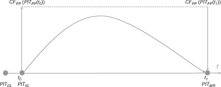
FIGURE 5.4 Cash flow pattern where the cash out-flow CFpp(PITvt) is expected to be returned as cash in-flow CFpp(PFTur)
we can define the different types by combining the quantity of principal amount within the corresponding PIT and TTC intervals.
5.3.1.1 Type I & II: Patterns of fixed principal amounts arising at fixed PIT and within fixed TTC iterations The pattern of fixed principal amounts appearing at fixed PIT and/or within fixed TTC iterations is driven by a deterministic set of contractual rules. Thus, the agreed exchange of the principal capital investment and the principal return defines such patterns. For instance, as illustrated in Figure 5.4, the cash outflow CF (PIT (t0)) agreed upon at deal time (PITdl) and provided by the lender at a predefined value time PITvl; moreover, the principal capital, defined as cash in-flow CFpp(PITpp(t1')), is expected to be returned from the borrower at the maturity point in time PITur. The exchange of the fixed cash “in” and “out” is expected within a predefined time cycle.
Within fixed cycle(s) there are expected cash flow patterns divided into a set of predefined fixed amounts according to the cycle iterations. Thus, principal payment cash flows paid at predefined TTC pattern are the step-ups fixed amounts for increasing the capital investment CFpp(1nc), provided by the lender as shown in Figure 5.5, and the fixed step-down amounts, illustrated in Figure 5.6, for decreasing the return notional amount of the loan5 CFPP(DEC>, expected from the borrower.
5.3.1.2 Type III & IV: Patterns of fixed principal cash-flows paid within variable PIT and TTC iterations These types of combinations are unlikely to appear under expected market conditions, counterparty characteristics and behavioral assumptions linked to contractually agreed terms. This is because the change in time dimensions, i.e., PIT and TTC, is very much linked and thus affects the principal payments and vice versa. However, under some unexpected “stress” conditions, a PIT, such as maturity time, may be shifted6 to an earlier or later point. However, as the duration of the contract changes, the expected amount of principal cash flows may stay the same. On the other hand, the maturity time and cycles of decreasing the principal, i.e., paying back from the borrower to the lender, will change accordingly. Figure 5.7 and Figure 5.8 illustrate the examples of time variation where the expected principal payments are applied.
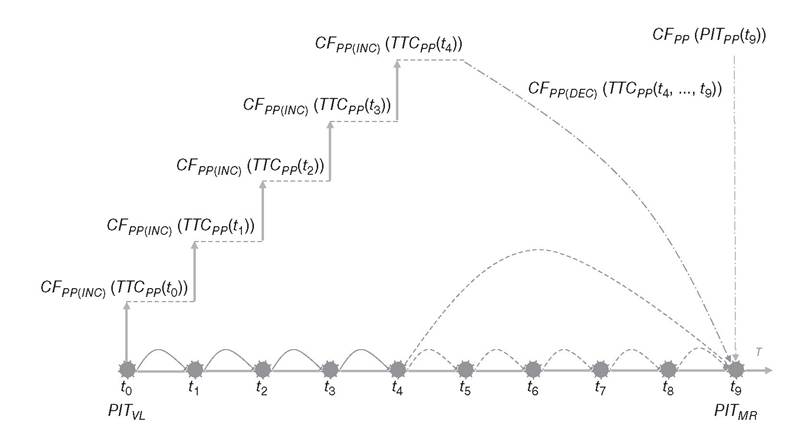
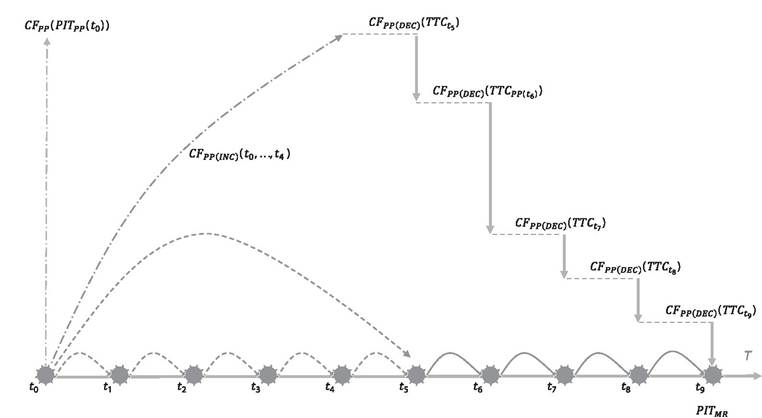
FIGURE 5.5 Expected cash flows of predefined fixed step-up principal amounts of capital investments, paid from predefined TTC time iterations divided by t0 to t4. The principal cash flow(s) from t5 to maturity time t9 could be based on a single amount, i.e., at t9 the CFpp(PlTpp(t9)), or on multiple divided amounts within TTC time iteration, i.e.,CFPP(DEC)(TTCPP(t5,..., t9)) as illustrated in Figure 5.6
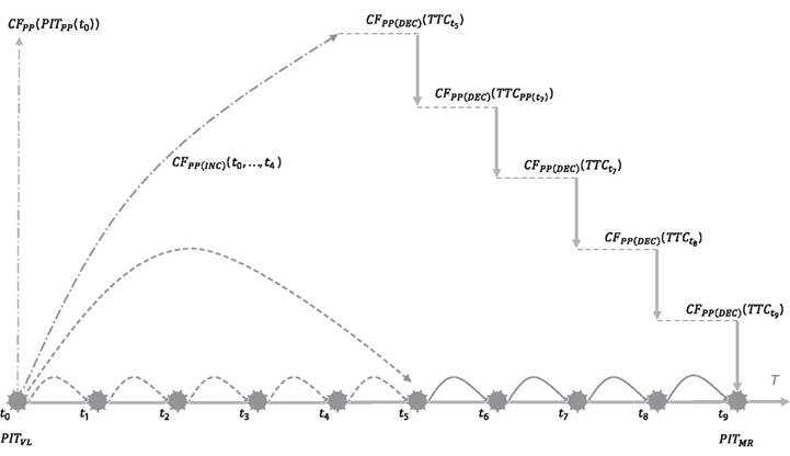
FIGURE 5.6 Expected cash flows of predefined fixed step-down principal return amounts, paid within predefined TTC time iteration, i.e., from t5 to maturity time at t9. The principal cash flows from t0 to t4 could be based on a single amount, i.e., at t0 the CFPP(PTTPP(t0)), or on multiple divided amounts within TTC time iteration, i.e., CFPP(!NCl(TTCPP(t0,..., t4)) as illustrated in Figure 5.5
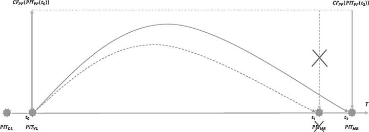
FIGURE 5.7 Cash flow pattern where the original maturity time PFTur is shifted and thus the cash in-flow CFpp(PTTpp)O2) is expected in a different time than originally agreed
5.3.1.3 Type V & VI: Patterns of variable principal amounts at fixed TTC and PIT There are some contracts where the principal amount may vary at set TTC or particular PIT.
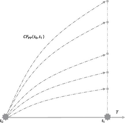
A typical case of variable principal amounts within fixed TTC iterations is the annuity loan, where the sum of interest and principle are equal until the maturity; in such contracts, the principal increase and the interest deteriorates through time. Moreover, the cash flow evolution of credit line patterns, also called facilities, fall into this category; in this case any credit amount, up to the line, could be used until a predefined PIT, e.g., 45 days. As illustrated in Figure 5.9 there are different cash flow patterns reflecting the lending of a principal amount within a cycle of time (t0, I1}; thus, at PIT, t1 the principal amount provided from the lender to the borrower may vary accordingly.There are instances where the amount of principal cash flows may change during the TTC iterations. A typical case of such a principal pattern is when a counterparty executes the contractually agreed upon option of pre-paying part of the remaining principal at some time before the maturity time. Thus, as illustrated in Figure 5.10, a prepayment event at t6 results in a reduction of the payment amount, set at t5.
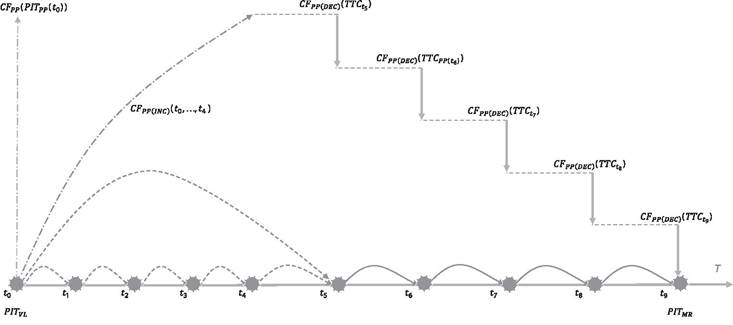
FIGURE 5.8 Step -down principal cash flows patterns of return amounts paid within modified TTC time iteration as maturity time is being extended (original pattern is as shown in Figure 5.6)
PITvl PITpp
FIGURE 5.9 Cash flow patterns representing the options of a borrower to lend principal capital, within a cycle of time {t0, t1}. At any particular PIT t1 when the borrower is using the credit facility, the principal amount may vary
PITvl
FIGURE 5.10 Variability of step-down principal return amounts due to prepayment event at t6, paid within predefined TTC time iteration, i.e., from t5 to maturity time at t9.
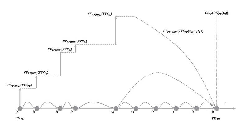
FIGURE 5.11 Cash flows of remaining principal amounts at step-up pattern driven by the credit needs within variable TTC time iterations from t0 to t4.
5.3.1.4 Type VII & VIII: Patterns of variable principal amounts at variable TTC and PIT This case is the one with the higher degree of flexibility (variability) in regards to the patterns of principal cash flows and PITs / TTC iterations. A typical pattern falling to these types is the cash flows of remaining principal amounts at step-ups driven by the credit requests within variable TTC time iterations; see for instance the example of such patterns of cash flow evolution from t0 to t4 as illustrated in Figure 5.11. This is very much applied in the loans where a defined principal capital has been agreed, however different amounts distributed through variable cycles are drawn according to the borrower’s credit needs, e.g., based on project evolution which is financed by the principal capital.
5.3.2 Interest patterns
In financial contracts representing a loan, the lender is expecting to earn an interest income, while the borrower sees interest as the price of getting credit. The two views are complementary and both parties should be able to understand and feel comfortable with the interest they have to receive or pay. Otherwise a loss or default may occur.
In terms of interest, it is important to understand the calculation parameters and the role of time in the payment process. Interest rates R(t), notional or principal amount of the loan, valuation rules, as well as time are the main ingredients that are combined to calculate interest.
The interest rate can be fixed and thus independent of future market conditions. It can also be set as variable which implies that the actual or assumed changes in market conditions will be considered where the corresponding rates will be reset at predefined time intervals, for example, quarterly. The patterns of the notional or principal amount, discussed earlier, are combined with interest rates to calculate the interest payments; for instance, by simply multiplying the interest rates with the notional or principal amount. A more complicated approach could be employed by applying interest capitalization. In this case, instead of being paid out, interest is capitalized and added to the outstanding principal.
Based on the definitions made in the contractual agreement the interest payments are expected at predefined points in time, e.g., at value or maturity date, or through the cycle time intervals, e.g., monthly, quarterly, etc. The measurement of time between financial events, e.g., the time (ti, ti+1) between two principal or interest payments, is a challenging issue in financial analysis. As discussed earlier, the duration of each month is an unequal pseudo-regular calendar based on day conventions such as A/A, A/365, 30/360, etc., used in the calculation of interest accruals over time.
The interest payments falling at particular PITs or TTC iterations during the lifetime of a non-defaulted financial contract define the pattern of interest cash flow events, denoted as CFpp. Interest payments can be fixed amounts. However, they normally vary TTC due to changes in principal and/or market evolution of interest rates. Interest payments are rather set at fixed PIT and TTC iterations; thus based on Table 5.1, we may expect the Type I, II, V and VI as discussed here.
5.3.2.1 Type I & II: Patterns of fixed interest occurring at fixed PIT and/or within fixed TTC iterations This is the case where fixed interest rates are applied whereas the principal amount is not changed until the maturity, as seen in Figure 5.12. Fixed interest TTC iterations could appear in fixed-rate bonds where the principal is paid at the maturity PIT. A zero coupon bond also has one fixed interest at maturity PIT.
5.3.2.2 Type V & VI: Patterns of variable interest occurring at fixed PIT and/or within fixed TTC iterations Mostinterestpaymentsarevariableduetocontractagreements referring to the type of interest rates, i.e., variable, and/or the evolution of the principal amount. In the former case, interest payments are fully dependent on the changes of rates within the future time terms. For instance, the interest cash flows of variable-rate bonds, paid TTC
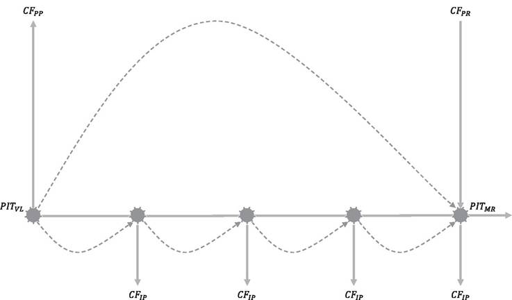
FIGURE 5.12 Equal Interest payments driven by fixed interest rates and steady principal amount
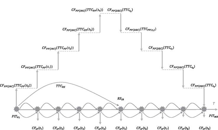
FIGURE 5.13 Cash flows of variable interest payments due to variable principles and interest rates
iterations, are expected not to be the same. In the latter case the future principal payments can be estimated or pre-defined, e.g., on annuity contracts or on loans with step-ups or step-downs as discussed earlier and illustrated in Figure 5.13. The example shown in this figure considers also the rate reset event TTCrs at t5. However, despite the type of interest rate, i.e., fixed or variable, applied in such contracts the interest payments are expected to be unequal within TTC iterations, due to principal changes.
5.3.3 Accrual interest patterns
There is a practical caveat in regards to interest that should be pointed out and carefully considered in interest calculations: the calculation of accrued interest payments that fall between the agreed time intervals. The borrower owes accrued to the lender, but has not paid them yet. The accrual over the interval beginning at tb and ending at tB is given by Equation 5.1.
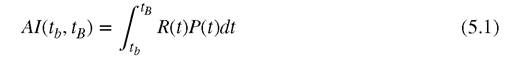
In practice, however, the principal and nominal interest rate change in a discreet rather than in a continuous manner and thus, Equation 5.1 can be simplified as shown in Equation 5.2 and Figure 5.14, where the accrual interest within the time intervals (ti, ti+1) is defined as follows:

where the interest rate R(t) and principal P(t) are constant in each segment.
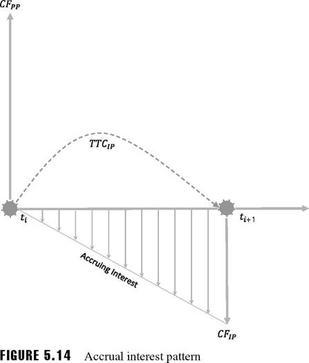
Note also that some important features are relevant to the correct calculation of accrual amounts. These are the capitalization of the interest, as mentioned above, the compounding method where implicit capitalization is assumed between successive interest payments and the upfront payment where interest is paid at the beginning of the accrual period instead of at its end.
5.3.2 Credit enhancements patterns
The cash flow events appearing after a credit event, i.e., counterparty default or downgrading, are results of the asset and/or counterparty based credit enhancements that we discuss in Chapter 10 (CreditEnhancements).
Particularly, for the assets based credit enhancements, the cash flow is a result of their liquidation.7 Thus, their value at the time of exercising them is the amount of cash flow used to cover the counterparty credit losses. As such assets are driven by market conditions, but also by the underlying counterparty credit status,8 their value may fluctuate over time and cannot be estimated precisely. Moreover, the exact time of such cash flows varies but is expected to occur shortly after the credit event assuming that the asset(s) are still liquid.
In the example shown in Figure 5.15, at t2 a default will cancel all future expected principal and interest cash flows. However, at some time after the default, e.g., tCE(1) and/or tCE(2), new cash flow(s) are expected from the credit enhancement(s). Both the amount and the time are estimated but under stressed conditions this could be rather imprecise.
When counterparty-based credit enhancements are used, the cash flows are expected from the guarantors or protection sellers after the counterparty credit risk event. The amount of
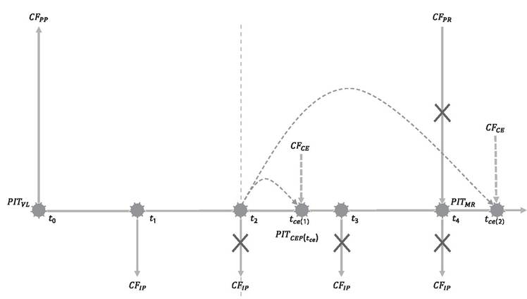
FIGURE 5.15 Cash flow of asset-based credit enhancements
the cash flows is expected to be equal to the value defined in the contractual agreements, i.e., guarantees or credit derivatives. The latter generates additional cash flow events referring to premiums paid to the protection seller until the maturity of the contract or until the time of the credit event. The time of the cash flows is normally defined in the contractual agreement9 but is expected usually later than the ones from the asset-based credit enhancements.
5.3.5 Behavior patterns
As already discussed, financial contracts contain a set of predefined rules used to estimate the financial events under given counterparty and market conditions. However, there are some rules which are driven by the behavior of the counterparty; for instance the counterparty may have an option to prepay a loan, withdrawing cash from a current account, drawdown the remaining principal amount of a loan or from a facility to fulfil possible liquidity needs.
In addition there is some unwritten behavior that must also be considered; counterparties may decide to cancel the financial contract, i.e., default, recover part of the outstanding credit exposure, or may also try to avoid default by using other loans. Such behavioral characteristics are discussed in Chapter 8 (Behavior Risk).
Behavior introduces to the analysis some unclear rules and unexpected events. Note, however, that financial analysis depends entirely on clear rules that are expected to be followed among the counterparties and creates the expected pattern of financial events. Practitioners therefore are mapping the behavior patterns by using replicating portfolios. Replication mimics the behavior of the counterparty by using well defined principal and interest patterns similar to the ones discussed in the above paragraphs. Such a technique is widely accepted and creates the basis for all types of financial analysis.
As we discuss in Chapter 8 (Behavior Risk), the main parameters considered in mapping the behavior are the amount and time. Note that it makes no sense to map the behavior at a
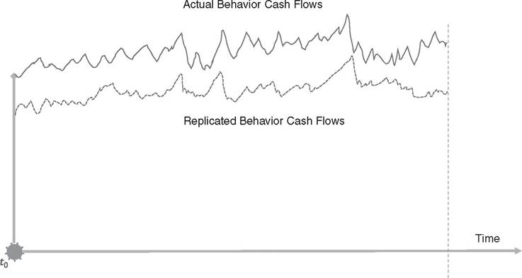
FIGURE 5.16 Example of actual and replicated behavior cash flows
single contract level; it is rather more practical to apply it at portfolio level as counterparties do behave in a similar manner. In replication portfolios, we are using financial contracts that take the role of shadow contracts and therefore substitute these two parameters. Take, for instance, the case of prepayment behavior where counterparties expected, statistically observed, to prepay an amount within a certain time horizon. A principal at maturity or annuity contract could mimic these expected cash flows.
Of course, different institutions may employ several replication portfolios to map the different behaviors of their customers and relative financial contracts. However, a perfect replication portfolio of mapping the behavior is very hard to construct (see an example in Figure 5.16). A good approach is to monitor the existing and mimic behaviors and adjust them later according to the current and future market and credit risk expectations. Under crisis and stress conditions the parameters of the replication portfolio should also be stressed accordingly. A well-defined replication portfolio should be able to align its stress parameters with the behavior stress factors.
5.3.3 Other patterns
In addition to the above, other patterns may also rise and be considered in the events' evolution of financial contracts, such as fees paid from obligors against prepayments, service fees, premiums that are agreed to be paid from protection buyers to protection sellers, dividends from stock and equities. These can be expected or unexpected financial events appearing at fixed or variable times, i.e., fall into one of the combinations defined in Table 5.1.
5.3.4 Example of financial events
Let us now describe a simple example illustrating financial events as shown in Figure 5.17. Let us assume a loan where at t0 of value date, indicated as PITvl, a principal amount cash-flow
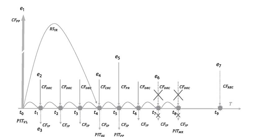
FIGURE 5.17 Example of financial events evolution
CFpp event, denoted as e1, is provided from the borrower to lender. At t1 to t8, the agreed principal payments CFdec and estimated interest payments CFip, paid from the lender to borrower, are the cash flow events denoted as e2 and e3 respectively; these events are expected to occur until the maturity date (PITmr) at t8. Moreover, the interest rate is reset RSir at PITRS of t4 and the loan is re-priced, e.g., based on the agreed corresponding referenced market conditions; such an event, denoted as e4, will result in a revaluation of the future interest payment cash-flows. At PITpp of t5 however, the lender decided to prepay part of the principal providing the corresponding cash flow CFpr. Such a prepayment event e5 may also affect the volume of the cash-flows for the future interest CFip and returns of principal payments. At t7 an unexpected default, denoted as e6, occurred; this implies that all future expected interest and principal cash flows, i.e., at t7 and t8, will be canceled out. However, at t9 a future event e7 may occur representing a cash flow due to expected recoveries CFrec and/or possible credit enhancements, e.g., collaterals, that may be exercised after the default event.
The degree of the number and type of financial events that will be generated in financial contracts depends on the richness and complexity of the rules defined in financial contracts and is linked to:
■ The type and number of market conditions, e.g., fixed or variable market expectations
■ The counterparties, e.g., degree of credit ratings
■ The behavior of the markets and counterparties, e.g., exercising the right to prepay
As we will see in Chapter 12, based on the financial events, the liquidity value, and income will be derived. Finally, the difference between the expected and unexpected performance of the input elements will influence the risk measurements in the output elements, such as funding and market liquidity risks, sensitivities, value and income at risk, together with the corresponding losses.
It is also important to understand that the cash flows of all contract types are received not only from the expected and unexpected future payments, e.g., principal, interest, etc., but also by the expected behavior, e.g., to get payments from recoveries and guarantors, as well as from the trading activities applied to financial collaterals. Still, we need to consider the different expectations in changes of market prices. Whether the contract holder is receiving these cash flows at the agreed time or unexpected future cycles or points in time, is fully dependent on market conditions, counterparties and corresponding behaviors to which the financial contract is linked.
5.4