TIME IN FINANCIAL CONTRACTS
In financial analysis, time plays a central role. This means that time exists as a background dimension within the entire financial system. However, there are two parallel time dimensions in financial analysis: one is about the exact times set in contractual agreement; it also defines the historical actual financial event and the present point in time (PIT) where the future starts.
The other dimension is the simulated and reported time. It refers to times, usually expressed as intervals, where we are considering the calculation and reporting of the financial events. Any calculation process of financial events follows this time dimension. Moreover, the estimation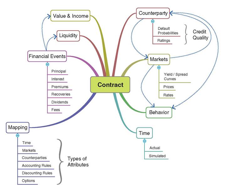
FIGURE 5.1 Main elements referring to financial contracts
of markets' evolution also considers such time dimensions. Dealing with the time dimension, we must also set the time where the analysis should start. This is for setting the point at which the pseudo-current (present) time analysis is defined and where the past and future periods are considered during the calculation process.
The rules defined are the agreement among counterparties that determines the what, how and when of a financial contract. In other words, what has to be done during the lifetime of the financial contract, how will it be done, and when? The when relates to two kinds of timing events. It is indicating a particular point in time (PIT) or through the cycle (TTC) iterations. This distinction informs the pattern of financial events in a contract.
In financial contracts, rules define the exact times at which actions are expected to be taken. PIT events indicate exact points in time that are non-recurring. Think for instance about the exact points when a contract starts and ends. TTC iterations represent the time cycles that are recurring, for example, when interest or principal payments will change hands between a borrower and a lender.
However, some timing events are less clearly defined. When a contract includes options that the counterparties can exercise at their convenience, timing assumptions are less accurate. An option of prepayment, for example, may be exercised according to a strategy or rational behavior that takes into account the future. In this case, we use a model that takes into account these time imprecise assumptions.The scale of the time can differ between minutes, hours, days, and years. The first two are only considered in intraday actions, such as trading activities, whereas the last two come into play in most short and longer term analysis. Using a time grid finer than daily can make most analytics almost impossible to use because, most likely, it increases the complexity of systems to a high degree.1 For this reason, time attributes defined in a contract are set on a daily grid or higher, e.g., week, month, quarter, etc. Moreover, in most market conditions, counterparty and behavior characteristics consider time on a daily or higher scale. The time buckets (defined usually as Time Bucket System TBS) used in financial analysis and the corresponding reports are set on single or combination of time intervals as Day(s), Week(s), Month(s), Quarter(s), Half-Year(s), and Year(s).
Even a daily grid can still make analytics overcomplicated. A gap analysis based only on daily buckets will demand expensive computation and will result in overly detailed reports. A contract with a duration of 10 years has almost 3,600 intervals when applying daily buckets, which will result in an amount of data that is impractical to work with. However, in the simulation process, daily intervals may have an important use. Financial analysts want to look at simulation results on a daily interval grid. To control liquidity, it is common to have daily intervals of about 30 days. On the other hand, the more detailed the simulation, the more expensive it becomes. Computation time is proportional to the number of simulated buckets.
Monthly buckets often suffice for most simulation. Long-term simulations might be done with even longer time intervals and lower precision. Keep in mind that accuracy and cost are a tradeoff. The longer the time interval, the less accurate is the forecast of market conditions, counterparty and behavior characteristics.But that is still not the entire story. When calendars define natural time in terms of days, weeks, months, and years, there are some special issues that have to be considered. Days have certain time intervals for trading, weeks may have five or six business days, months have between 28 and 31 days2 and years may be common or leap. All this becomes an issue when we are constructing algorithms that need to be accurate over several years or even decades. In many cases, the duration of each month is simplified to be considered as 30 days, i.e., January and February are both treated the same. Such a pseudo-regular calendar introduces errors in the analysis that are invisible on a monthly basis. Thus, for instance, daily basis in the analysis raises issues in calculating correctly the accrual on the 31st day of January. In addition, leap years introduce additional complexity when interest is accrued over years. Thus, financial analysts use different day count conventions such as A/A, A/365,30/360ISDA, 30E/360, 30/365, etc. Based on these conventions, interest accrues over time, and it can be determined more accurately. Moreover, exact quantification of time intervals is important in the discounting process.
Figure 5.2 illustrates the main elements of time discussed above.
5.3