DEFAULT PROBABILITY

All counterparties have a probability of default (PD), even though it might be very low. Defining this probability is a complex exercise as there is a need for combining quantitative and qualitative information, historical data and future assumptions of the market risk factors.

Default probability is the fundamental counterparty risk factor, which indicates the like­lihood for the counterparty to default. Despite the existence of such probabilities, as long as there are no default events the contractual events, such as the expected cash flows, still occur as expected. Obviously the survival is complementary to default probability.

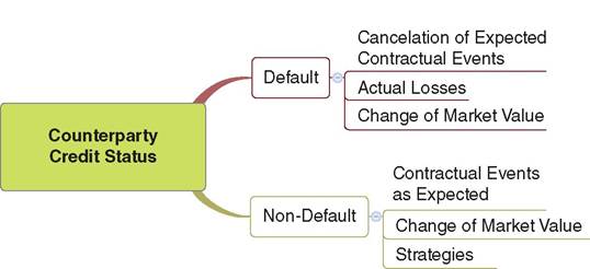
FIGURE 7.2 Impacts of default and non-default statuses

Regardless, default probabilities impact the market value of the financial contract through ratings and discounting credit spreads; it also drives the funding contingent strategies of the credit portfolio, explained in Chapter 12. Of course a default event immediately turns the status of counterparty to “default” which results in the cancelation of the expected financial events and actual credit losses, as explained in Chapters 5 and 9, whereas it impacts directly the value of the contract and portfolio that it belongs to.

There are two types of models applied to identify and estimate default and survival probabilities named structural and intensity (also called reduced form) models.

7.3.1 Structural models

Structural models¹ estimate the likelihood of default by considering the economic funda­mentals of a counterparty, e.g., company's debt and equity ratio. The value, V, of a firm at future time, t, is uncertain, due to many external and internal factors (economic risk, busi­ness risk, foreign exchange risk, industry risk, etc.). Structural models therefore are based on measurable endogeneous and exogenous parameters, which impact the counterparty's value and inherently impact the financial capability to repay the debt. Thus, such models are mainly applied in corporate/company types of counterparty.

Following Merton's model, a firm's value V_t assumes the returns on its assets distributed normally and their behavior can be described with Brownian motion formulation:

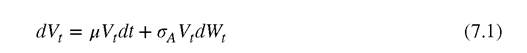
with V (0) = V₀, W is a Brownian motion (random value taken from standardized normal distribution), σA is a constant assets volatility and μ a constant drift.

Consequently, the firm's assets value, assumed to obey a lognormal diffusion process with a constant volatility, is given by

The debt value at t < T with debt maturity, T, a debt face value L, and a possible company default at T is,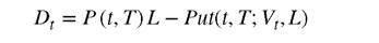

where P (t, T) L is the discounted face value and Put (t, T; V_t, Lj is a put option with underlying V and strike L

The default probability is

Note, however, that Merton's model does not allow for a premature default, in the sense that the default may only occur at the maturity of the claim.

Employing KMV Model, a default even is likely to appear when the firm's asset values reach a certain level defined as threshold, which could before the maturity date T. This threshold for defaulting is set as “Default Point” which is roughly approximated by the sum of all the Short Term Debt (STD) and half of the Long Term Debt (LTD).

Then, an index called Distance to Default (DD) defines the distance between the expected assets value of the firm within an analysis horizon, and the default point, normalized by standard deviation of the future asset returns.

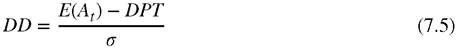
Such distance to default can be calculated as absolute or relative value. The former is the sum of initial distance and the growth of that distance within the period T:

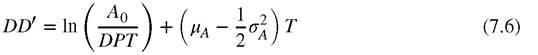
with μA drift rate, defining the expected rate of return of the firm's asset and σA the volatility of the underlying asset.

An extended approach to Merton's model, assuming that default actually can happen before the maturity date, is proposed by Black and Cox. In this model a time dependent safety barrier, H (t), is introduced. Thus, the default either occurs when the value of firm's assets hits a lower threshold or at maturity date T. However, if the value starts away from the default barrier then the degree of survival probabilities tends, very quickly, to be equal to one. Another challenge is to specify the lower threshold appropriately. Thus, there are extensions of the Black and Cox Model where Barrier change may also be randomly employed.^2,3

In the Hull and White structural model the default probabilities are consistent with those implied by bond prices and CDS spreads and where the joint probability of default across a large number of counterparties can be sampled from a multivariate normal distribution.

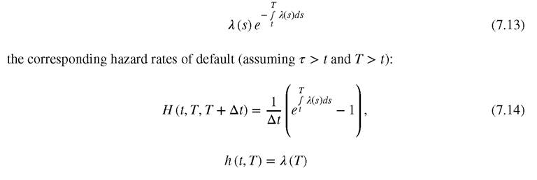
In such approach the Hazard Function is defined by credit indices (quality) and can be assumed to be driven by standard Brownian Motion. Moreover, given that default has not occurred by time t, the interpretation of the hazard rate represents the conditional probability of the occurrence of default in a small time interval [t,t+dt].

7.3.2 Intensity models

In the intensity (also called reduced form) based credit risk models the risk of default event probability arrives exogenously. By employing an intensity model we attempt to model the pattern with which defaults arrive, rather than explain them endogenously. In such models, the implied default probability over a (small) time interval is modelled as proportional to the length of the time interval. The frequency of the events arriving in the time interval [t, t + Δt) is described by a number called the intensity, denoted as λ (t).

The risk of default event is modelled via a counting process N (t):

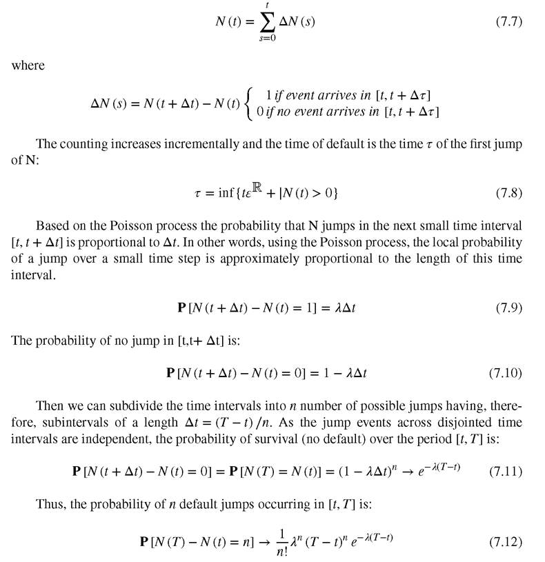
The intensity λ is the hazard rate which is driving the default probability.

The first jump of the Poisson process, however, is a rather rare event. In order to achieve a more realistic model the default intensity and therefore hazard rate must be changed more dynamically through the time. The inhomogeneous Poisson process therefore has been intro­duced where the density of the time of the first jump, given that no jump has occurred until t is:

In the above paragraphs we highlight the main advantages and elements of most commonly used intensity and structural models. A more detailed description of these models can be found in Annex B, which is available on the website. In marketplace lending where the information referring to endogenous parameters of the counterparties is limited we propose that intensity rather structural models are more appropriate to be applied in defining default probabilities.

Default probabilities drive their usage in risk management and pricing of the credit portfolio. This means that, similar to the market expectation, a clear distinction between the risk-neutral and real-world default probabilities should be made.

7.3.3 Real-world and risk-neutral default probabilities

In Chapter 6 we discussed the real-world and risk-neutral expectations in regards to markets. Similarly, we now consider real-world and risk-neutral default probabilities. Both views and corresponding analysis serve different and complementary purposes.

As in the analysis of real-world market expectations, real-world default probabilities can be determined through empirical studies, historical observations and assumptions for defining scenario generator models of future credit events. Such real-world future default probabilities are very much applicable in risk management analysis. Indeed, real-world default probabilities are quantitatively assessing and measuring the probability of the counterparty to default, based on certain quantitative scenarios, and their impact on the outcomes of value and liquidity. In other words, it is defining the sensitivity of value, income and liquidity against the default credit events.

We have already discussed risk-neutral probabilities where we assume the absence of arbitrage; thus, unlike in the real world, the risk-neutral default probabilities are the basis of pricing approaches similar to the concept followed in market arbitrage-free models. Never­theless, why are real default probabilities not part of such approaches? The answer lies in the expected behavior of investors who tend to avoid any possible losses. Let's imagine, for example, an investment where the expected outcomes are $100 with probability 99% and $0 with “default” probability of 1%. Investors with non-rational behavior would enter into such a deal, with a price of $99,⁴ as the expected return has much higher probability than the one with entire loss.

After all, investments are adjusting the instruments that are not risk-free by including in the discounting risk-free factors, e.g., interest rate r the real-world default probabilities, i.e., expressed as credit spreads ³ that reflect the additional risk and resulting losses. The additive spreads will obviously impact directly on the expected cash flows and value⁶ of the financial contracts.

7.4