THE RISK-NEUTRAL EXPECTATIONS

Based on risk-neutral expectations, one can price using discount rates and applying high analytical approaches which result in well-defined, expected payoffs. Yield curves and forward rates and prices are the fundamental elements applied in the space of risk-neutral expectations.

6.3.1 Yield curves

A yield curve is a discount rate curve, with each point on the curve representing the discount average rates of discounting, starting from today and travelling along the points on the time axis. Because it is an average-rate curve, it tends to be smooth, even using linear or spline interpolations.

Yield curves may have different curve slopes and directions based on the expected market conditions, and they come in four basic shapes as illustrated in Figure 6.2:

■ Normal: where the curve slopes gently upwards, usually at relatively short term

■ Upwards (rising or positive) sloping: where the yield is historically a low level but the long rates are significantly greater than the short rates

■ Downwards (inverted or negative) sloping: where the yield is historically a high level but the long rates are significantly lower than the short rates

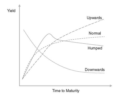
FIGURE 6.2 Example of basic shapes of yield curves

■ Humped: where yield curves are rising upwards, reaching the peak point at medium term, and then sloping downwards

Investors should act in line with their expectations. For instance, in the case of expecting a rise of short-term interest rates, they should only buy short-term loans and at maturity roll over the investment. It is safe to say that roughly 80-90 percent of yield curves have positive slopes.

Intuitively, we can say that short-term maturity investments are less risky than those with a longer maturity.

In peer-to-peer lending, lenders and borrowers have much less flexibility. Most loan terms are medium, e.g., 36 to 60 months, with fixed interest rates. These loans are still relatively shorter-term compared to a 30-year mortgage. Regardless, if a lender invests in an illiquid product with a duration of five years and ends up being stuck in this investment in times of adverse market conditions, the illiquidity of these assets can become a problem.

6.3.2 Forward rates and prices

Forward rates¹ can be defined as the way the market feels about the movements of interest rates in the future. They do this by extrapolating from the risk-free theoretical spot rates which cannot actually be observed directly from the market. A forward rate curve is a curve of normal short-term rates as seen at different points in time in the future. For example, it is possible to calculate the one-year forward rate one year from now. Thus, to compute a bond's value using forward rates, you must first calculate this rate. After you have calculated this value, you just plug it into the formula for the prices of a bond where the interest rate or yield would be inserted.

Forward rates are calculated from current market rates following mathematical principles to establish what the market believes based on the arbitrage-free rates for dealing today, or at analysis date, at rates that are effective at some point in the future. The absence of arbitrage is one of the most important axioms in mathematical finance. It helps us to work out the price of simple contracts such as retail loans and deposits to derivative instruments.

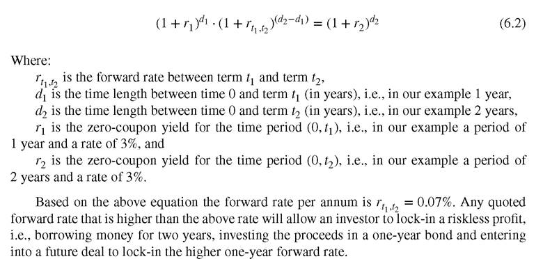
The absence of arbitrage is based on the market mechanism of adjusting supply and demand. However, it can occur locally and for short periods of time. As soon as arbitrage opportunities exceed a certain threshold, risk seekers find arbitrage opportunities. The threshold is determined by the costs of arbitrage, which means that in practice, only highly organized investors for whom these costs are minimal can profit from arbitrage opportunities. Such opportunities still exist in well-developed liquid markets.

Finally, forward rates are driven by market expectations and cannot fully predict future rates. The forward rate calculated in the above example of 0.07% may differ from the expected economic forecast for the one-year. In fact, if you compare the actual rates within a term structure of let's say three months with the forward rate curve for the same term structure, the rates will certainly not differ much.

If we interpret the forward rates as the economically expected future spot rate, interest rates should be rising most of the time. Yet, this is not necessarily true; the observed rates typically revert to a medium and longer-term mean. Arbitrage-free models of interest rate dynamics are well structured and mathematically well defined; however they are unable to economically forecast the interest rates, at least not in the medium and long term.

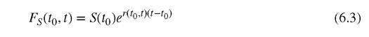
The modelling and estimation of forward prices and forward exchange rates are relatively simple and rather straightforward. Knowing that spot prices are observed we can say that at the time t the forward price of a stock F_s(t₀, t) with current price S(t₀) is given by 6.3:

In regards to the forward exchange rates,² we need to consider the interest rate term structure of both domestic and foreign currencies that need to be exchanged. Thus, based on the current Foreign Exchange rate FX(t₀) and the difference of the domestic and foreign spot interest rates Δr(t₀, t) with term t, the equation for estimating the t-forward exchange rate is given by 6.4:

In the above equation 6.4 the forward premium equals the difference between domestic and foreign interest rates which is based on the assumption of interest rate parity under arbitrage-free conditions.

The reason we even bring up commodities in this context is that they may be collateral in a loan contract and the market may wish to price them. The estimation of the commodities’ forward prices has some additional complexity due to the fact that we should also consider their storage³ cost as well as the incapability for making available for consuming or producing within a short time; the latter issue makes the short selling very difficult which almost vanishes arbitrage opportunities. Thus, similarly to 6.3, at time t the forward price of a commodity F_c(t₀, t) with current price C(t₀) is given by 6.5:

Note that in the exponential factor of the above arbitrage-free pricing formula of commod­ity forward prices 6.5 the additional term c represents the storage cost whereas the term cy, named convenience yield, represents the adjustment to the cost of carry, a physical commodity, which for instance is keeping a production process active.

Even though practitioners use forward rates and prices, we should remember that they cannot predict future spot prices or future spot exchange rates. This is due to the fact that forward rates or prices are not economic forecasted rates. Instead, they are based on arbitrage- free conditions that lead to biased forecasting. The economic dynamics that influence the future interest rates or prices play no role in determining the forward price and rates. In fact future interest rates or prices are not only dependent on the market (investors) expectations of the future returns but also on the volatility and unexpected performance of this return, i.e., on the riskiness and future uncertainties. Considering real-world expectations allows a more realistic analysis of future investment performance.

6.4