UNDERLYING ASSUMPTIONS OF THE ANALYSIS
Marketplace loans are, in effect, simple annuity contracts. We explained the structure of expected financial events of annuities in Chapter 5 (5.3 Contract Mechanisms Producing Financial Events) and their risk (market and credit defaults).
These are the steps we applied in the model.13.1.1 Gettingtheinputdata
We use the following information provided by Lending Club: counterparty id, principal amount, value date, duration of the contract, cycle of payments, interest rates, and counterparty ratings and sub-ratings.
13.1.2 Time
The analysis date is set on 1 January 2014. The Time Bucket System for the simulation intervals is defined as monthly to align with the actual contractual time intervals.
13.1.3 Risk factors
Based on the above data, we set the following model parameters for the market, counterparty and behavior risks:
■ Market parameters are only referring to market interest and credit spread rates. They are used for discounting and they drive expected cash flows, value and income.
■ All counterparties have a rating—A, B, C, D, E, F and G—from best to worst. Each rating class has five sub-ratings, such as A1 to A5, B1 to B5 and so forth.
■ Ratings drive default probabilities, spreads and recovery rates.
■ We consider two behavior characteristics: prepayments and recoveries in case of default.
13.1.4 Mapping the financial contract
We derive the amortization schedule of the payments by using a fixed rate annuity contract type for mapping the financial contract. The main attributes of such contract are:
■ Value date (starting point of the contract)
■ Principal amount (present value of the loan), set value date
■ Annual interest rates
■ Cycle of interest and principal payment derived by the number of payment periods and the total duration of the loan
13.1.5 Calculating contractual financial events
The computation engine provides all financial events including all expected cash flows, values and incomes at both points in time and through the cycle iterations.
13.1.6 Constructingportfolios
Based on the available provided data of the contractual deals, we randomly generate 1,000 portfolios containing 1,000 contracts each. For each contract of these portfolios, the model calculates all financial events.
13.1.7 Analysis outputs
We perform liquidity, value, exposure, profit and loss analysis at the contract and portfolio level under canonical conditions and two different stress scenarios—A and B—with different levels of stress. The model generates several types of report.
Figure 13.1 illustrates the layout of this model. It includes most of the considerations about profitability and analysis that we outlined in Part Two of this book.
In the following paragraphs, we describe the results of the model in more detail. Without intending to spoil the surprise, we conclude that returns are good when conditions stay as they are. As soon as defaults rise under modest stress, portfolio returns decrease to low single-digit returns over the holding period, or turn negative.
We are unsure if investors are in a position to perform analytics as described in Part Two of this book. Risk management (i.e., by performing stress testing) could help platforms offer advice to investors to optimize their portfolios.
Table 13.1 shows the results of the return distribution of three scenarios under canonical (ideal) conditions and the two different stress scenarios, both annualized and for the full duration of the holding period. Scenario A applies “mild stress,” Scenario B applies “medium stress.” This table shows the changes in portfolio performance under the different scenarios. We will explain the underlying assumptions of each scenario under the heading “Stress test scenarios.”
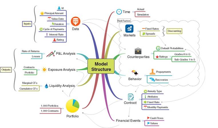
FIGURE 13.1 Layoutofthemodel
TABLE 13.1 Summary statistics of the model portfolio under canonical conditions and stress conditions
| Scenario | Mean | Standard Deviation | Median | Skewness | Kurtosis | |||||
| Full Duration | Annual | Full Duration | Annual | Full Duration | Annual | Full Duration | Annual | Full Duration | Annual | |
| Canonical | 23.8979 | 6.6262 | 0.2068 | 0.0090 | 23.8962 | 6.6262 | 0.0898 | 0.0386 | 2.7082 | 2.9557 |
| Scenario A | 4.0136 | 1.4286 | 0.0378 | 0.0091 | 4.0129 | 1.4287 | -0.0230 | -0.0194 | 3.0609 | 2.9392 |
| Scenario B | -14.7135 | -4.0096 | 0.1002 | 0.0171 | -14.7105 | -4.0094 | -0.0920 | -0.1130 | 2.7321 | 2.8617 |
A more in-depth conclusion follows at the end of this chapter.
Let's now go through the model parameters and analysis of this model step by step. Figure 13.1 shows the layout of the model.13.2